9 Confidence Intervals

Definition: Confidence Interval

A confidence interval gives a range of plausible values for a parameter. It depends on a specified confidence level with higher confidence levels corresponding to wider confidence intervals and lower confidence levels corresponding to narrower confidence intervals. Common confidence levels include 90%, 95%, and 99%.

Usually we don’t just begin chapters with a definition, but confidence intervals are simple to define and play an important role in the sciences and any field that uses data. You can think of a confidence interval as playing the role of a net when fishing. Instead of just trying to catch a fish with a single spear (estimating an unknown parameter by using a single point estimate/statistic), we can use a net to try to provide a range of possible locations for the fish (use a range of possible values based around our statistic to make a plausible guess as to the location of the parameter).

Needed packages

Let’s load all the packages needed for this chapter (this assumes you’ve already installed them). If needed, read Section 2.3 for information on how to install and load R packages.

library(dplyr)
library(ggplot2)
library(mosaic)
library(knitr)
library(ggplot2movies)

9.1 Bootstrapping

Just as we did in Chapter 10 with the Lady Tasting Tea when making hypotheses about a population total with which we would like to test which one is more plausible, we can also use computation to infer conclusions about a population quantitative statistic such as the mean. In this case, we will focus on constructing confidence intervals to produce plausible values for a population mean. (We can do a similar analysis for a population median or other summary measure as well.)

Traditionally, the way to construct confidence intervals for a mean is to assume a normal distribution for the population or to invoke the Central Limit Theorem and get, what often appears to be magic, results. (This is similar to what was done in Section 10.8.) These methods are often not intuitive, especially for those that lack a strong mathematical background. They also come with their fair share of assumptions and often turn Statistics, a field that is full of tons of useful applications to many different fields and disciplines, into a robotic procedural-based topic. It doesn’t have to be that way!

In this section, we will introduce the concept of bootstrapping. It will be a useful tool that will allow us to estimate the variability of our statistic from sample to sample. One neat feature of bootstrapping is that it enables us to approximate the sampling distribution and estimate the distribution’s standard deviation using ONLY the information in the one selected (original) sample. It sounds just as plagued with the magical type qualities of traditional theory-based inference on initial glance but we will see that it provides an intuitive and useful way to make inferences, especially when the samples are of medium to large size.

To introduce the concept of bootstrapping, we again will use the movies dataset in the ggplot2movies data frame. Recall that you can also glance at this data frame using the View function and look at the help documentation for movies using the ? function. We will explore many other features of this dataset in the chapters to come, but here we will be focusing on the rating variable corresponding to the average IMDB user rating.

You may notice that this dataset is quite large: 58,788 movies have data collected about them here. This will correspond to our population of ALL movies. Remember from Chapter ?? that our population is rarely known. We use this dataset as our population here to show you the power of bootstrapping in estimating population parameters. We’ll see how confidence intervals built using the bootstrap distribution perform at including our population parameter of interest. Here we can actually calculate these values since our population is known, but remember that in general this isn’t the case.

Let’s take a look at what the distribution of our population ratings looks like. We’ll see that we will use the distribution of our sample(s) as an estimate of this population histogram.

movies %>% ggplot(aes(x = rating)) +
  geom_histogram(color = "white", bins = 20)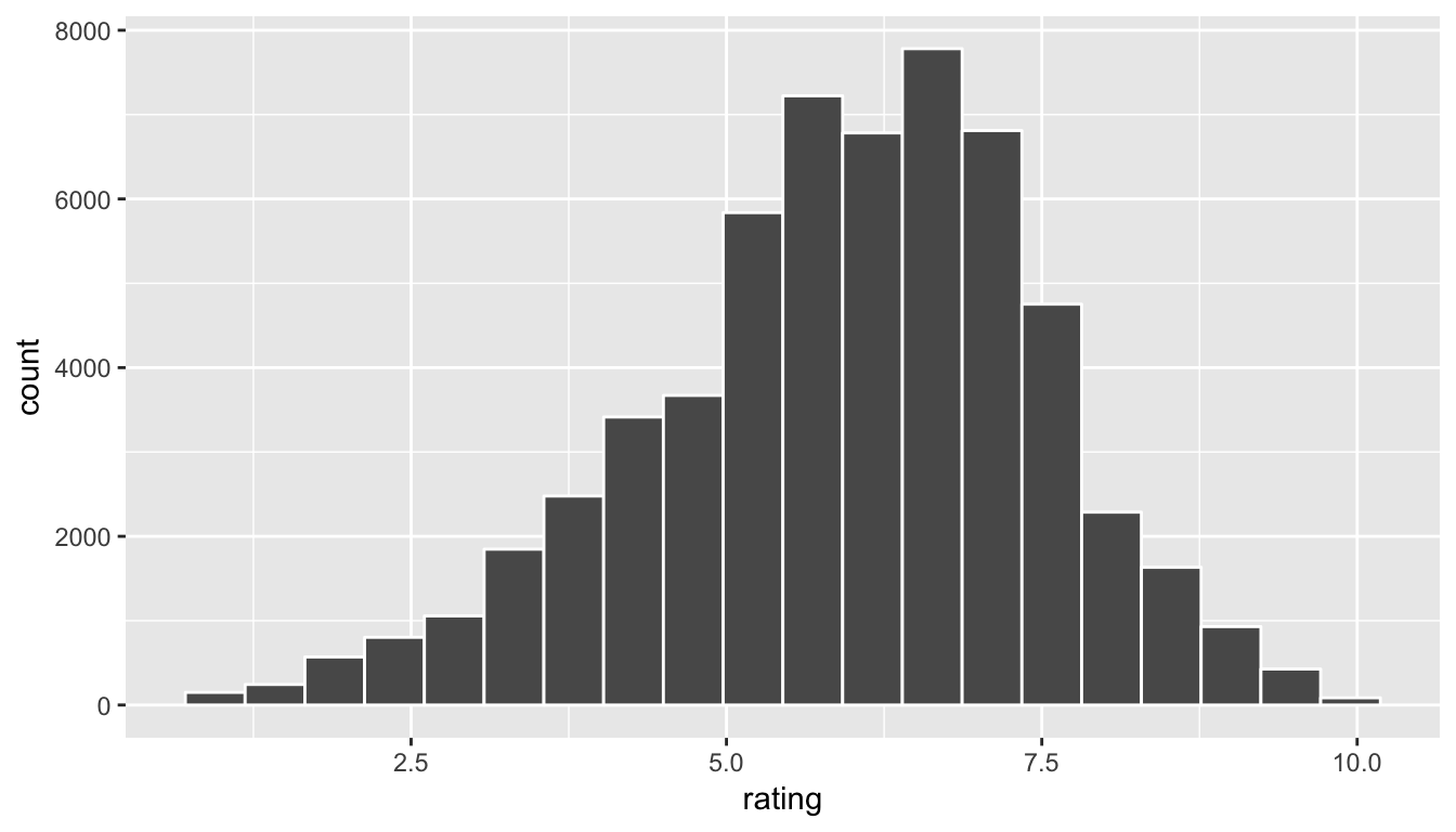

Figure 9.1: Population ratings histogram

Learning check

(LC9.1) Why was a histogram chosen as the plot to make for the rating variable above?

(LC9.2) What does the shape of the rating histogram tell us about how IMDB users rate movies? What stands out about the plot?

It’s important to think about what our goal is here. We would like to produce a confidence interval for the population mean rating. We will have to pretend for a moment that we don’t have all 58,788 movies. Let’s say that we only have a random sample of 50 movies from this dataset instead. In order to get a random sample, we can use the resample function in the mosaic package with replace = FALSE. We could also use the sample_n function from dplyr.

set.seed(2017)
movies_sample <- movies %>% 
  sample_n(50)

The sample_n function has filtered the data frame movies “at random” to choose only 50 rows from the larger movies data frame. We store information on these 50 movies in the movies_sample data frame.

Let’s now explore what the rating variable looks like for these 50 movies:

ggplot(data = movies_sample, aes(x = rating)) +
  geom_histogram(color = "white", bins = 20)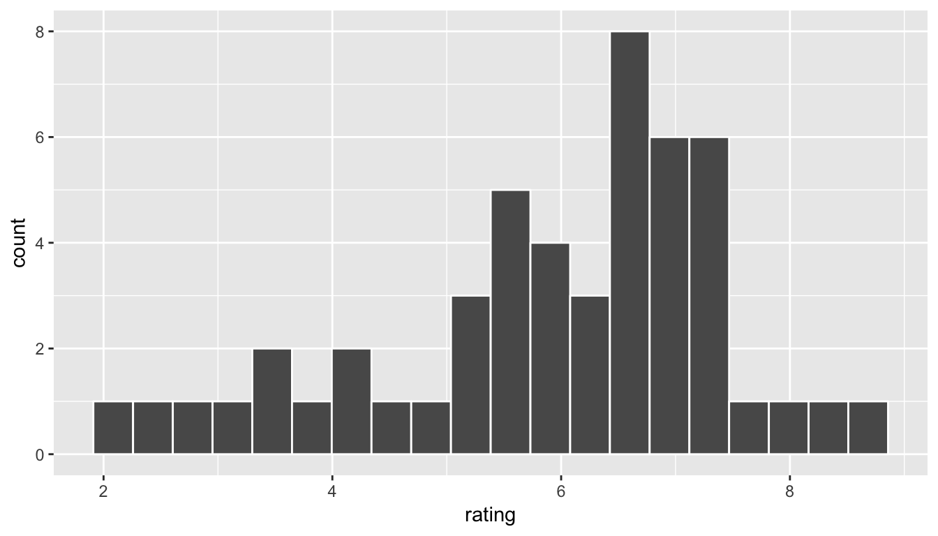

Figure 9.2: Sample ratings histogram

Remember that we can think of this histogram as an estimate of our population distribution histogram that we saw above. We are interested in the population mean rating and trying to find a range of plausible values for that value. A good start in guessing the population mean is to use the mean of our sample rating from the movies_sample data:

(movies_sample_mean <- movies_sample %>% 
   summarize(mean = mean(rating)))

# A tibble: 1 x 1
   mean
  <dbl>
1  5.89

Note the use of the ( ) at the beginning and the end of this creation of the movies_sample_mean object. If you’d like to print out your newly created object, you can enclose it in the parentheses as we have here.

This value of 5.894 is just one guess at the population mean. The idea behind bootstrapping is to sample with replacement from the original sample to create new resamples of the same size as our original sample.

Returning to our example, let’s investigate what one such resample of the movies_sample dataset accomplishes. We can create one resample/bootstrap sample by using the resample function in the mosaic package.

boot1 <- resample(movies_sample) %>%
  arrange(orig.id)

The important thing to note here is the original row numbers from the movies_sample data frame in the far right column called orig.ids. Since we are sampling with replacement, there is a strong likelihood that some of the 50 observational units are going to be selected again.

You may be asking yourself what does this mean and how does this lead us to creating a distribution for the sample mean. Recall that the original sample mean of our data was calculated using the summarize function above.

Learning check

(LC9.3) What happens if we change the seed to our pseudo-random generation? Try it above when we used resample to describe the resulting movies_sample.

(LC9.4) Why is sampling at random important from the movies data frame? Why don’t we just pick Action movies and do bootstrapping with this Action movies subset?

(LC9.5) What was the purpose of assuming we didn’t have access to the full movies dataset here?

Before we had a calculated mean in our original sample of 5.894. Let’s calculate the mean of ratings in our bootstrapped sample:

(movies_boot1_mean <- boot1 %>% summarize(mean = mean(rating)))

# A tibble: 1 x 1
   mean
  <dbl>
1  5.69

More than likely the calculated bootstrap sample mean is different than the original sample mean. This is what was meant earlier by the sample means having some variability. What we are trying to do is replicate many different samples being taken from a larger population. Our best guess at what the population looks like is multiple copies of the sample we collected. We then can sample from that larger “created” population by generating bootstrap samples.

Similar to what we did in the previous section, we can repeat this process using the do function followed by an asterisk. Let’s look at 10 different bootstrap means for ratings from movies_sample. Note the use of the resample function here.

do(10) * 
  (resample(movies_sample) %>% 
     summarize(mean = mean(rating)))

You should see some variability begin to tease its way out here. Many of the simulated means will be close to our original sample mean but many will stray pretty far away. This occurs because outliers may have been selected a couple of times in the resampling or small values were selected more than larger. There are myriad reasons why this might be the case.

So what’s the next step now? Just as we repeated the repetitions thousands of times with the “Lady Tasting Tea” example, we can do a similar thing here:

trials <- do(5000) * summarize(resample(movies_sample), mean = mean(rating))

ggplot(data = trials, mapping = aes(x = mean)) +
  geom_histogram(bins = 30, color = "white")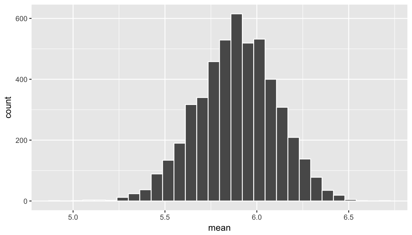

Figure 9.3: Bootstrapped means histogram

The shape of this resulting distribution may look familiar to you. It resembles the well-known normal (bell-shaped) curve. At this point, we can easily calculate a confidence interval. In fact, we have a couple different options. We will first use the percentiles of the distribution we just created to isolate the middle 95% of values. This will correspond to our 95% confidence interval for the population mean rating, denoted by \(\mu\).

(ciq_mean_rating <- confint(trials, level = 0.95, method = "quantile"))

  name lower upper level     method estimate
1 mean  5.46   6.3  0.95 percentile     5.89

It’s always important at this point to interpret the results of this confidence interval calculation. In this context, we can say something like the following:

Based on the sample data and bootstrapping techniques, we can be 95% confident that the true mean rating of ALL IMDB ratings is between 5.46 and 6.3.

This statement may seem a little confusing to you. Another way to think about this is that this confidence interval was constructed using the sample data by a procedure that is 95% reliable in that of 100 generated confidence intervals based on 100 different random samples, we expect on average that 95 of them will capture the true unknown parameter. This also means that we will get invalid results 5% of the time. Just as we had a trade-off with \(\alpha\) and \(\beta\) with hypothesis tests, we have a similar trade-off here with setting the confidence level.

To further reiterate this point, the graphic below from Diez, Barr, and Çetinkaya-Rundel (2014) shows us that if we repeated a confidence interval process 25 times with 25 different samples, we would expect about 95% of them to actually contain the population parameter of interest. This parameter is marked with a dotted vertical line. We can see that only one confidence interval does not overlap with this value. (The one marked in red.) Therefore 24 in 25 (96%), which is quite close to our 95% reliability, do include the population parameter.

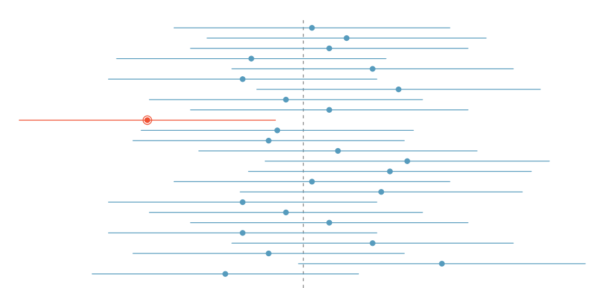
Figure 9.4: Confidence interval coverage plot from OpenIntro

Remember that we are pretending like we don’t know what the mean IMDB rating for ALL movies is. Our population here is all of the movies listed in the movies data frame from ggplot2movies. So does our bootstrapped confidence interval here contain the actual mean value?

movies %>% summarize(mean_rating = mean(rating))

# A tibble: 1 x 1
  mean_rating
        <dbl>
1        5.93

We see here that the population mean does fall in our range of plausible values generated from the bootstrapped samples.

We can also get an idea of how the theory-based inference techniques would have approximated this confidence interval by using the formula \[\bar{x} \pm (2 * SE),\] where \(\bar{x}\) is our original sample mean and \(SE\) stands for standard error and corresponds to the standard deviation of the bootstrap distribution. The value of 2 here corresponds to it being a 95% confidence interval. (95% of the values in a normal distribution fall within 2 standard deviations of the mean.) This formula assumes that the bootstrap distribution is symmetric and bell-shaped. This is often the case with bootstrap distributions, especially those in which the original distribution of the sample is not highly skewed.

Definition: standard error

The standard error is the standard deviation of the sampling distribution. The sampling distribution may be approximated by the bootstrap distribution or the null distribution depending on the context. Traditional theory-based methodologies for inference also have formulas for standard errors, assuming some conditions are met.

To compute this type of confidence interval, we only need to make a slight modification to the confint function seen above. (The expression after the \(\pm\) sign is known as the margin of error.)

(cise_mean_rating <- confint(trials, level = 0.95, method = "stderr"))

  name lower upper level method estimate margin.of.error
1 mean  5.47  6.32  0.95 stderr     5.89           0.425

Based on the sample data and bootstrapping techniques, we can be 95% confident that the true mean rating of ALL IMDB ratings is between 5.467 and 6.316.

Learning check

(LC9.6) Reproduce the bootstrapping above using a sample of size 50 instead of 25. What changes do you see?

(LC9.7) Reproduce the bootstrapping above using a sample of size 5 instead of 25. What changes do you see?

(LC9.8) How does the sample size affect the analysis above?

(LC9.9) Why must bootstrap samples be the same size as the original sample?

9.1.1 Review of bootstrapping

We can summarize the process to generate a bootstrap distribution here in a series of steps that clearly identify the terminology we will use (R. Lock et al. 2012).

Generate bootstrap samples by sampling with replacement from the original sample, using the same sample size.
Compute the statistic of interest, called a bootstrap statistic, for each of the bootstrap samples.
Collect the statistics for many bootstrap samples to create a bootstrap distribution.

Visually, we can represent this process in the following diagram.

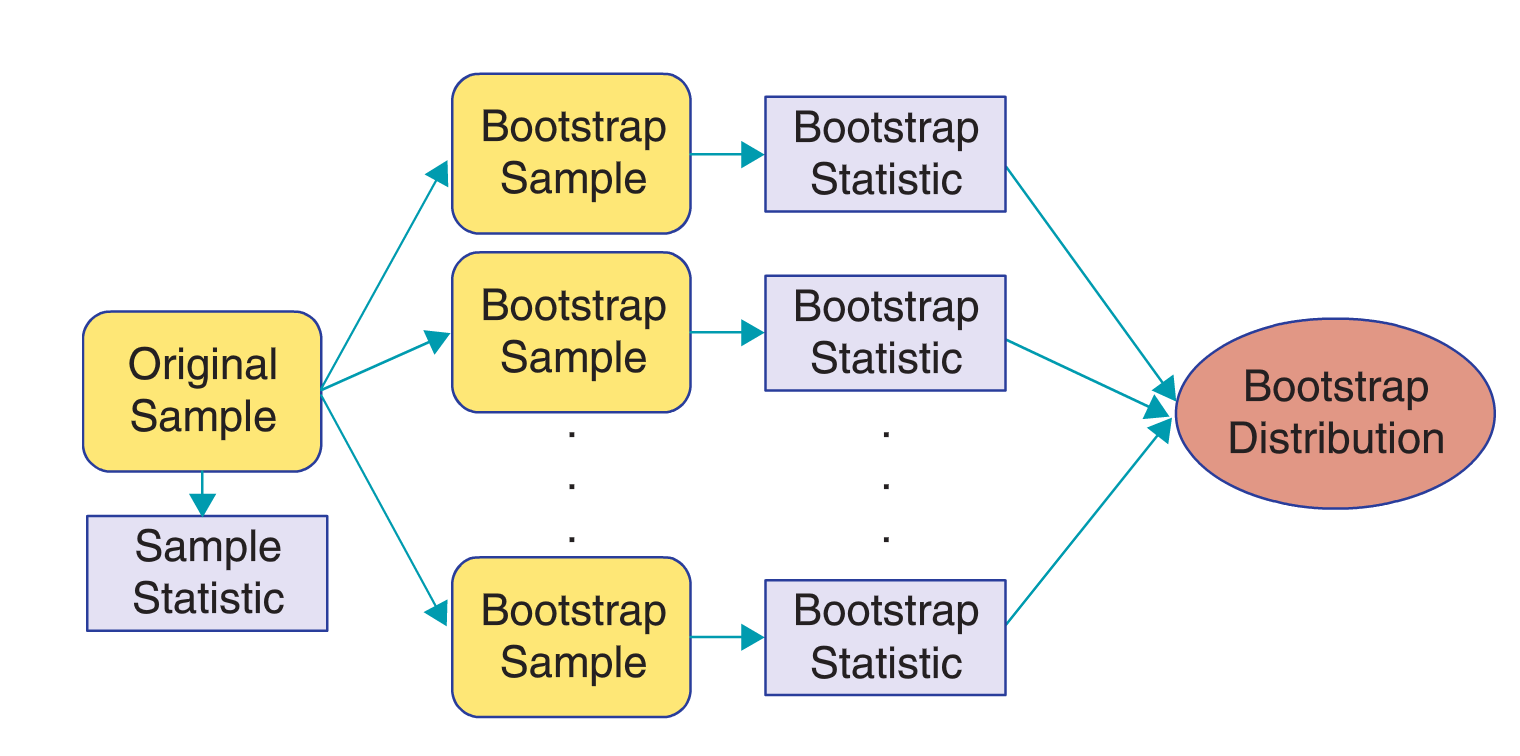
Figure 9.5: Bootstrapping diagram from Lock5 textbook

9.2 Relation to hypothesis testing

Recall that we found a statistically significant difference in the sample mean of romance movie ratings compared to the sample mean of action movie ratings. We concluded Chapter 10 by attempting to understand just how much greater we could expect the population mean romance movie rating to be compared to the population mean action movie rating. In order to do so, we will calculate a confidence interval for the difference \(\mu_r - \mu_a\). We’ll then go back to our population parameter values and see if our confidence interval contains our parameter value.

We could use bootstrapping in a way similar to that done above, except now on a difference in sample means, to create a distribution and then use the confint function with the option of quantile to determine a confidence interval for the plausible values of the difference in population means. This is an excellent programming activity and the reader is urged to try to do so.

Recall what the randomization/null distribution looked like for our simulated shuffled sample means:

Note all this code was moved over from hypothesis testing

(movies_trimmed <- movies %>% select(title, year, rating, Action, Romance))

# A tibble: 58,788 x 5
   title                     year rating Action Romance
   <chr>                    <int>  <dbl>  <int>   <int>
 1 $                         1971   6.40      0       0
 2 $1000 a Touchdown         1939   6.00      0       0
 3 $21 a Day Once a Month    1941   8.20      0       0
 4 $40,000                   1996   8.20      0       0
 5 $50,000 Climax Show, The  1975   3.40      0       0
 6 $pent                     2000   4.30      0       0
 7 $windle                   2002   5.30      1       0
 8 '15'                      2002   6.70      0       0
 9 '38                       1987   6.60      0       0
10 '49-'17                   1917   6.00      0       0
# ... with 58,778 more rows

movies_trimmed <- movies_trimmed %>%
  filter(!(Action == 1 & Romance == 1))

movies_trimmed <- movies_trimmed %>%
  mutate(genre = ifelse(Action == 1, "Action",
                        ifelse(Romance == 1, "Romance",
                               "Neither"))) %>%
  filter(genre != "Neither") %>%
  select(-Action, -Romance)

set.seed(2017)
movies_genre_sample <- movies_trimmed %>% 
  group_by(genre) %>%
  sample_n(34) %>% 
  ungroup()

mean_ratings <- movies_genre_sample %>% 
  group_by(genre) %>%
  summarize(mean = mean(rating))
obs_diff <- diff(mean_ratings$mean)

shuffled_ratings <- #movies_trimmed %>%
  movies_genre_sample %>% 
     mutate(genre = shuffle(genre)) %>% 
     group_by(genre) %>%
     summarize(mean = mean(rating))
diff(shuffled_ratings$mean)

[1] -0.132

set.seed(2017)
many_shuffles <- do(5000) * 
  (movies_genre_sample %>% 
     mutate(genre = shuffle(genre)) %>% 
     group_by(genre) %>%
     summarize(mean = mean(rating))
   )

rand_distn <- many_shuffles %>%
  group_by(.index) %>%
  summarize(diffmean = diff(mean))
head(rand_distn, 10)

# A tibble: 10 x 2
   .index diffmean
    <dbl>    <dbl>
 1   1.00 -0.132  
 2   2.00 -0.197  
 3   3.00 -0.0265 
 4   4.00  0.715  
 5   5.00 -0.474  
 6   6.00 -0.121  
 7   7.00 -0.174  
 8   8.00 -0.209  
 9   9.00 -0.00882
10  10.0  -0.332

ggplot(data = rand_distn, mapping = aes(x = diffmean)) +
  geom_histogram(color = "white", bins = 20)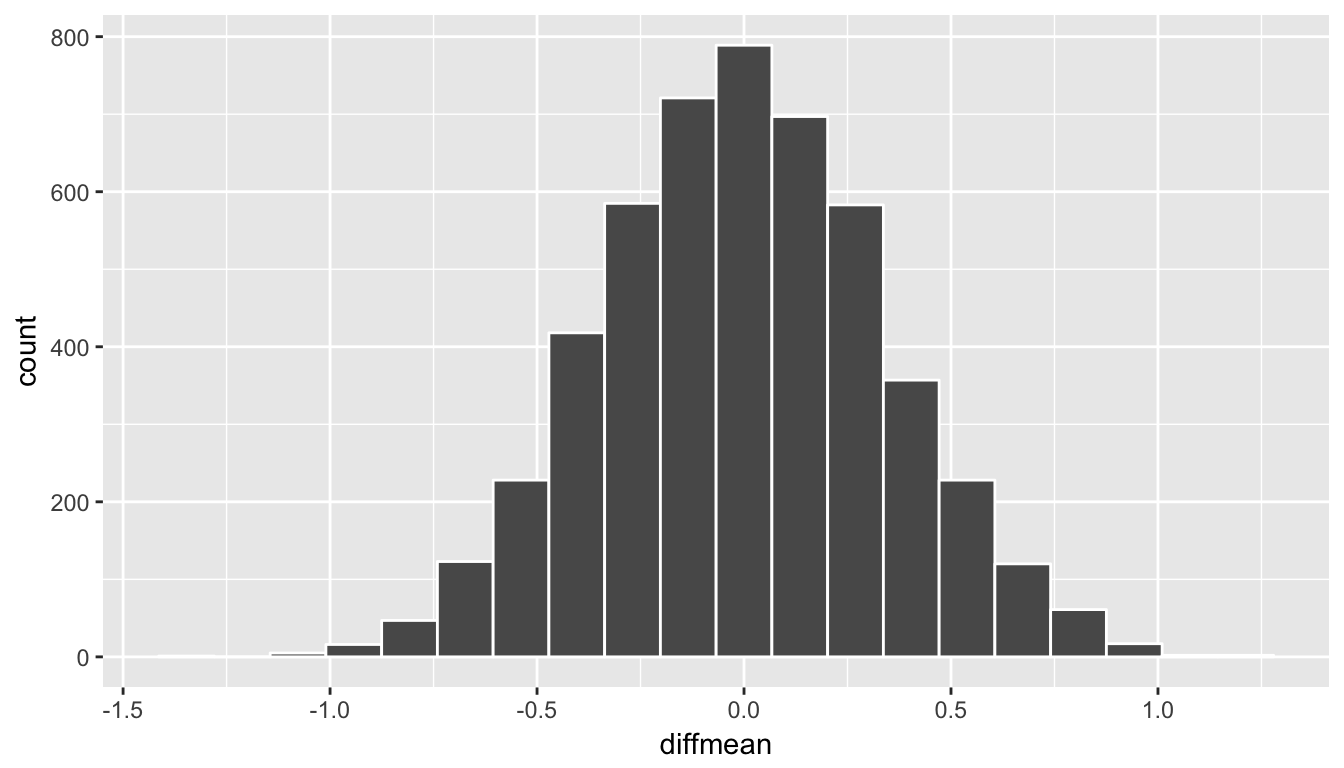

Figure 9.6: Simulated shuffled sample means histogram

With this null distribution being quite symmetric and bell-shaped, the standard error method introduced above likely provides a good estimate of a range of plausible values for \(\mu_r - \mu_a\). Another nice option here is that we can use the standard deviation of the null/randomization distribution we just found with our hypothesis test.

(std_err <- rand_distn %>% summarize(se = sd(diffmean)))

# A tibble: 1 x 1
     se
  <dbl>
1 0.340

We can use the general formula of \(statistic \pm (2 * SE)\) for a confidence interval to obtain the following result for plausible values of the difference in population means at the 95% level.

(lower <- obs_diff - (2 * std_err))

     se
1 0.269

(upper <- obs_diff + (2 * std_err))

    se
1 1.63

We can, therefore, say that we are 95% confident that the population mean rating for romance movies is between 0.269 and 1.631 points higher than for that of action movies.

The important thing to check here is whether 0 is contained in the confidence interval. If it is, it is plausible that the difference in the two population means between the two groups is 0. This means that the null hypothesis is plausible. The results of the hypothesis test and the confidence interval should match as they do here. We rejected the null hypothesis with hypothesis testing and we have evidence here that the mean rating for romance movies is higher than for action movies.

9.3 Effect size

The phrase effect size has been thrown around recently as an alternative to \(p\)-values. In combination with the confidence interval, it can be often more valuable than just looking at the results of a hypothesis test. It depends on the scientific discipline exactly what is meant by “effect size” but, in general, it refers to the magnitude of the difference between group measurements. For our two sample problem involving movies, it is the observed difference in sample means obs_diff.

It’s worthy of mention here that confidence intervals are always centered at the observed statistic. In other words, if you are looking at a confidence interval and someone asks you what the “effect size” is you can simply find the midpoint of the stated confidence interval.

Learning check

(LC9.10) Check to see whether the difference in population mean ratings for the two genres falls in the confidence interval we found here. Are we guaranteed that it will fall in the range of plausible values?

(LC9.11) Why do you think many scientific fields are shifting to preferring inclusion of confidence intervals in articles over just \(p\)-values and hypothesis tests?

(LC9.12) Why is 95% related to a value of 2 in the margin of error? What would approximate values be for 90% and for 99%?

(LC9.13) Why is a 95% confidence interval wider than a 90% confidence interval? Explain by using a concrete example from everyday life about what is meant by “confidence.”

(LC9.14) How would confidence intervals correspond to one-sided hypothesis tests?

(LC9.15) There is a relationship between the significance level and the confidence level. What do you think it is?

(LC9.16) The moment the phrase “standard error” is mentioned, there seems to be someone that says “The standard error is \(s\) divided by the square root of \(n\).” This standard error formula is used in the theory-based procedure for an inference on one mean. But… does it always work? For samp1, samp2, and samp3 below, do the following:

produce a bootstrap distribution based on the sample
calculate the standard deviation of the bootstrap distribution
compare this value of the standard error to what you obtain when you calculate the standard deviation of the sample \(s\) divided by \(\sqrt{n}\).

df1 <- data_frame(samp1 = rexp(50))
df2 <- data_frame(samp2 = rnorm(100))
df3 <- data_frame(samp3 = rbeta(20, 5, 5))

Describe how \(s / \sqrt{n}\) does in approximating the standard error for these three samples and their corresponding bootstrap distributions.

9.4 Conclusion

9.4.1 What’s to come?

This concludes the Inference unit of this book. You should now have a thorough introduction into topics in both data science and statistics. In the last chapter of the textbook, we’ll summarize the purpose of this book as well as present an excellent example of what goes into making an effective story via data.

9.4.2 Script of R code

An R script file of all R code used in this chapter is available here.