
2 Getting Started with Data in R
Before we can start exploring data in R, there are some key concepts to understand first:
- What are R and RStudio?
- How do I code in R?
- What are R packages?
If you are already familiar with these concepts, feel free to skip to Section 2.4 below introducing some of the datasets we will explore in depth in this book. Much of this chapter is based on two sources which you should feel free to use as references if you are looking for additional details:
- Ismay’s Getting used to R, RStudio, and R Markdown (Ismay 2016), which includes video screen recordings that you can follow along and pause as you learn.
- DataCamp’s online tutorials. DataCamp is a browser-based interactive platform for learning data science and their tutorials will help facilitate your learning of the above concepts (and other topics in this book). Go to DataCamp and create an account before continuing.
2.1 What are R and RStudio?
For much of this book, we will assume that you are using R via RStudio. First time users often confuse the two. At its simplest:
- R is like a car’s engine
- RStudio is like a car’s dashboard
| R: Engine | RStudio: Dashboard |
|---|---|
 |
 |
More precisely, R is a programming language that runs computations while RStudio is an integrated development environment (IDE) that provides an interface by adding many convenient features and tools. So the way of having access to a speedometer, rearview mirrors, and a navigation system makes driving much easier, using RStudio’s interface makes using R much easier as well.
Optional: For a more in-depth discussion on the difference between R and RStudio IDE, watch this DataCamp video (2m52s).
2.1.1 Installing R and RStudio
If your instructor has provided you with a link and access to RStudio Server, then you can skip this section. We do recommend though after a few months of working on the RStudio Server that you return to these instructions. If you don’t know what RStudio Server is, then please continue.
You will first need to download and install both R and RStudio (Desktop version) on your computer.
- Download and install R.
- Note: You must do this first.
- Click on the download link corresponding to your computer’s operating system.
- Download and install RStudio.
- Scroll down to “Installers for Supported Platforms”
- Click on the download link corresponding to your computer’s operating system.
Optional: If you need more detailed instructions on how to install R and RStudio, watch this DataCamp video (1m22s).
2.1.2 Using R via RStudio
Recall our car analogy from above. Much as we don’t drive a car by interacting directly with the engine but rather by using elements on the car’s dashboard, we won’t be using R directly but rather we will use RStudio’s interface. After you install R and RStudio on your computer, you’ll have two new programs AKA applications you can open. We will always work in RStudio and not R. In other words:
| R: Do not open this | RStudio: Open this |
|---|---|
 |
 |
After you open RStudio, you should see the following:
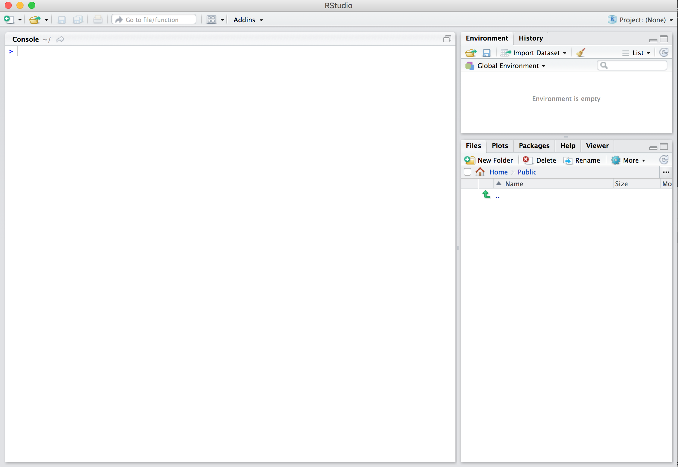
Watch the following DataCamp video (4m10s) to learn about the different panes in RStudio, in particular the Console pane where you will later run R code.
2.2 How do I code in R?
Now that you’re set up with R and RStudio, you are probably asking yourself “OK. Now how do I use R?” The first thing to note as that unlike other software like Excel, STATA, or SAS that provide point and click interfaces, R is an interpreted language, meaning you have to enter in R commands written in R code i.e. you have to program in R (we use the terms “coding” and “programming” interchangeably in this book).
While it is not required to be a seasoned coder/computer programmer to use R, there is still a set of basic programming concepts that R users need to understand. Consequently, while this book is not a book on programming, you will still learn just enough of these basic programming concepts needed to explore and analyze data effectively.
2.2.1 Basic programming concepts needed
To introduce you to many of these basic programming concepts, we direct you to the following DataCamp online interactive tutorials. For each of the tutorials, we give a list of the basic programming concepts covered. Note that in this book, we will use a different font to distinguish regular font from computer code.
It is important to note that while these tutorials serve as excellent introductions, a single pass through them is insufficient for long-term learning and retention. The ultimate tools for long-term learning and retention are “learning by doing” and repetition, something we will have you do over the course of the entire book and we encourage this process as much as possible as you learn any new skill.
- From the Introduction to R course complete the following chapters. As you work through the chapters, carefully note the important terms and what they are used for. We recommend you do so in a notebook that you can easily refer back to.
- Chapter 1 Intro to basics:
- Console pane: where you enter in commands
- Objects: where values are saved, how to assign values to objects.
- Data types: integers, doubles/numerics, logicals, characters.
- Chapter 2 Vectors:
- Vectors: a series of values.
- Chapter 4 Factors:
- Categorical data (as opposed to numerical data) are represented in R as
factors.
- Categorical data (as opposed to numerical data) are represented in R as
- Chapter 5 Data frames:
- Data frames are analogous to rectangular spreadsheets: they are representations of datasets in R where the rows correspond observations and the columns correspond to variables that describe the observations. We will revisit this later in Section 2.4.
- Chapter 1 Intro to basics:
- From the Intermediate R course complete the following chapters:
- Chapter 1 Conditionals and Control Flow:
- Testing for equality in R using
==(and not=which is typically used for assignment). Ex:2 + 1 == 3compares2 + 1to3and is correct R syntax, while2 + 1 = 3is not and is incorrect R syntax. - Boolean algebra:
TRUE/FALSEstatements and mathematical operators such as<(less than),<=(less than or equal), and!=(not equal to). - Logical operators:
&representing “and”,|representing “or”. Ex:(2 + 1 == 3) & (2 + 1 == 4)returnsFALSEwhile(2 + 1 == 3) | (2 + 1 == 4)returnsTRUE.
- Testing for equality in R using
- Chapter 3 Functions:
- Concept of functions: they take in inputs (called arguments) and return outputs.
- You either manually specify a function’s arguments or use the function’s defaults.
- Chapter 1 Conditionals and Control Flow:
This list is by no means an exhaustive list of all the programming concepts needed to become a savvy R user; such a list would be so large it wouldn’t be very useful, especially for novices. Rather, we feel this is the bare minimum you need to know before you get started; the rest we feel you can learn as you go. Remember that your knowledge of all of these concepts will build as you get better and better at “speaking R” and getting used to its syntax.
2.2.2 Tips on learning to code
Learning to code/program is very much like learning a foreign language, it can be very daunting and frustrating at first. However just as with learning a foreign language, if you put in the effort and are not afraid to make mistakes, anybody can learn. Lastly, there are a few useful things to keep in mind as you learn to program:
- Computers are stupid: You have to tell a computer everything it needs to do. Furthermore, your instructions can’t have any mistakes in them, nor can they be ambiguous in any way.
- Do not code from scratch: Especially when learning a new programming language, it is often much easier to taking existing code and modify it, rather than trying to write new code from scratch. So please take the code we provide throughout this book and play around with it!
- Practice is the key: You won’t get better if you don’t continue to practice working with the skills you are learning in R. Just as you can’t go months without speaking a new foreign language, you can’t go long periods of time without practice in R and catch on. We recommend you set aside at least a few minutes a day to R practice by doing.
2.3 What are R packages?
An R package is a collection of functions, data, and documentation that extends the capabilities of R. They are written by a world-wide community of R users. For example, among the many packages we will use in this book are the
However, there are two key things to remember about R packages:
- Installation: Most packages are not installed by default when you install R and RStudio. You need to install a package before you can use it. Once you’ve installed it, you likely don’t need to install it again unless you want to update it to a newer version of the package.
- Loading: Packages are not loaded automatically when you open RStudio. You need to load them everytime you open RStudio.
2.3.1 Package installation
(Note that if you are working on an RStudio Server, you probably will not need to install your own packages as that has been already done for you. Still it is important that you know this process for later when you are not using the RStudio Server but rather your own installation of RStudio Desktop.)
There are two ways to install an R package. For example, to install the ggplot2 package:
- In the Files pane:
- Click on “Packages”
- Click on “Install”
- Type the name of the package under “Packages (separate multiple with space or comma):” In this case, type
ggplot2 - Click “Install”
- Alternatively, in the Console pane run
install.packages("ggplot2")(you must include the quotation marks).
Repeat this for the dplyr package.
Note: You only have to install a package once, unless you want to update an already installed package to the latest version. If you want to update a package to the latest version, then re-install it by repeating the above steps.
2.3.2 Package loading
After you’ve installed a package, you can now load it using the library() command. For example, to load the ggplot2 and dplyr packages, run the following code in the Console pane:
library(ggplot2)
library(dplyr)Note: You have to reload each package you want to use every time you open a new session of RStudio. This is a little annoying to get used to and will be your most common error as you begin. When you see an error such as
Error: could not find functionremember that this likely comes from you trying to use a function in a package that has not been loaded. Remember to run the library() function with the appropriate package to fix this error.
2.4 Exploring real data
Let’s put everything we’ve learned so far into practice and start exploring some real data! Data comes to us in a variety of formats, from pictures to text to numbers. Throughout this book, we’ll focus on datasets that can be stored in a spreadsheet as that is among the most common way data is collected in the many fields. Remember from Subsection 2.2.1 that these “spreadsheet”-type datasets are called data frames in R and we will focus on working with data frames throughout this book.
Let’s first load all the packages needed for this chapter (This assumes you’ve already installed them. Read Section 2.3 for information on how to install and load R packages if you haven’t already.) At the beginning of all subsequent chapters in this text, we’ll always have a list of packages similar to what follows that you should have installed and loaded to work with that chapter’s R code.
library(dplyr)
library(nycflights13)
library(knitr)
2.4.1 nycflights13 package
We likely have all flown on airplanes or know someone who has. Air travel has become an ever-present aspect in many people’s lives. If you live in or are visiting a relatively large city and you walk around that city’s airport, you see gates showing flight information from many different airlines. And you will frequently see that some flights are delayed because of a variety of conditions. Are there ways that we can avoid having to deal with these flight delays?
We’d all like to arrive at our destinations on time whenever possible. (Unless you secretly love hanging out at airports. If you are one of these people, pretend for the moment that you are very much anticipating being at your final destination.) Throughout this book, we’re going to analyze data related to flights contained in the nycflights13 package (Wickham 2017). Specifically, this package contains five datasets saved as “data frames” (see Section 2.2) with information about all domestic flights departing from New York City in 2013, from either Newark Liberty International (EWR), John F. Kennedy International (JFK), or LaGuardia (LGA) airports:
flights: information on all 336,776 flightsairlines: translation between two letter IATA carrier codes and names (16 in total)planes: construction information about each of 3,322 planes usedweather: hourly meteorological data (about 8710 observations) for each of the three NYC airportsairports: airport names and locations
2.4.2 flights data frame
We will begin by exploring the flights data frame that is included in the nycflights13 package and getting an idea of its structure. Run the following in your code in your console: it loads in the flights dataset into your Console. Note depending on the size of your monitor, the output may vary slightly.
flights# A tibble: 336,776 x 19
year month day dep_time sched_dep_time dep_delay arr_time sched_arr_time
<int> <int> <int> <int> <int> <dbl> <int> <int>
1 2013 1 1 517 515 2.00 830 819
2 2013 1 1 533 529 4.00 850 830
3 2013 1 1 542 540 2.00 923 850
4 2013 1 1 544 545 -1.00 1004 1022
5 2013 1 1 554 600 -6.00 812 837
6 2013 1 1 554 558 -4.00 740 728
7 2013 1 1 555 600 -5.00 913 854
8 2013 1 1 557 600 -3.00 709 723
9 2013 1 1 557 600 -3.00 838 846
10 2013 1 1 558 600 -2.00 753 745
# ... with 336,766 more rows, and 11 more variables: arr_delay <dbl>, carrier
# <chr>, flight <int>, tailnum <chr>, origin <chr>, dest <chr>, air_time
# <dbl>, distance <dbl>, hour <dbl>, minute <dbl>, time_hour <dttm>Let’s unpack this output:
A tibble: 336,776 x 19: atibbleis a kind of data frame. This particular data frame has336,776rows19columns corresponding to 19 variables describing each observation
year month day dep_time sched_dep_time dep_delay arr_timeare different columns, in other words variables, of this data frame.- We then have the first 10 rows of observations corresponding to 10 flights.
... with 336,766 more rows, and 11 more variables:indicating to us that 336,766 more rows of data and 11 more variables could not fit in this screen.
Unfortunately, this output does not allow us to explore the data very well. Let’s look at different tools to explore data frames.
2.4.3 Exploring data frames
Among the many ways of getting a feel for the data contained in a data frame such as flights, we present three functions that take as their argument the data frame in question:
- Using the
View()function built for use in RStudio. We will use this the most. - Using the
glimpse()function loaded viadplyrpackage - Using the
kable()function in theknitrpackage - Using the
$operator to view a single variable in a data frame
1. View():
Run View(flights) in your Console in RStudio and explore this data frame in the resulting pop-up viewer. You should get into the habit of always Viewing any data frames that come your way.
Note the capital “V” in View. R is case-sensitive so you’ll receive an error is you run view(flights) instead of View(flights).
Learning check
(LC2.1) What does any ONE row in this flights dataset refer to?
- A. Data on an airline
- B. Data on a flight
- C. Data on an airport
- D. Data on multiple flights
Learning Check Solutions
(LC2.1) What does any ONE row in this flights dataset refer to? This is data on a flight. Not a flight path! Example:
- a flight path would be United 1545 to Houston
- a flight would be United 1545 to Houston 2013/1/1 at 5:15am
By running View(flights), we see the different variables listed in the columns and we see that there are different types of variables. Some of the variables like distance, day, and arr_delay are what we will call quantitative variables. These variables are numerical in nature. Other variables here are categorical.
Note that if you look in the leftmost column of the View(flights) output, you will see a column of numbers. These are the row numbers of the dataset. If you glance across a row with the same number, say row 5, you can get an idea of what each row corresponds to. In other words, this will allow you to identify what object is being referred to in a given row. This is often called the observational unit. The observational unit in this example is an individual flight departing New York City in 2013. You can identify the observational unit by determining what the thing is that is being measured in each of the variables.
2. glimpse():
The second way to explore a data frame is using the glimpse() function that you can access after you’ve loaded the dplyr package. It provides us with much of the above information and more.
glimpse(flights)Observations: 336,776
Variables: 19
$ year <int> 2013, 2013, 2013, 2013, 2013, 2013, 2013, 2013, 2013...
$ month <int> 1, 1, 1, 1, 1, 1, 1, 1, 1, 1, 1, 1, 1, 1, 1, 1, 1, 1...
$ day <int> 1, 1, 1, 1, 1, 1, 1, 1, 1, 1, 1, 1, 1, 1, 1, 1, 1, 1...
$ dep_time <int> 517, 533, 542, 544, 554, 554, 555, 557, 557, 558, 55...
$ sched_dep_time <int> 515, 529, 540, 545, 600, 558, 600, 600, 600, 600, 60...
$ dep_delay <dbl> 2, 4, 2, -1, -6, -4, -5, -3, -3, -2, -2, -2, -2, -2,...
$ arr_time <int> 830, 850, 923, 1004, 812, 740, 913, 709, 838, 753, 8...
$ sched_arr_time <int> 819, 830, 850, 1022, 837, 728, 854, 723, 846, 745, 8...
$ arr_delay <dbl> 11, 20, 33, -18, -25, 12, 19, -14, -8, 8, -2, -3, 7,...
$ carrier <chr> "UA", "UA", "AA", "B6", "DL", "UA", "B6", "EV", "B6"...
$ flight <int> 1545, 1714, 1141, 725, 461, 1696, 507, 5708, 79, 301...
$ tailnum <chr> "N14228", "N24211", "N619AA", "N804JB", "N668DN", "N...
$ origin <chr> "EWR", "LGA", "JFK", "JFK", "LGA", "EWR", "EWR", "LG...
$ dest <chr> "IAH", "IAH", "MIA", "BQN", "ATL", "ORD", "FLL", "IA...
$ air_time <dbl> 227, 227, 160, 183, 116, 150, 158, 53, 140, 138, 149...
$ distance <dbl> 1400, 1416, 1089, 1576, 762, 719, 1065, 229, 944, 73...
$ hour <dbl> 5, 5, 5, 5, 6, 5, 6, 6, 6, 6, 6, 6, 6, 6, 6, 5, 6, 6...
$ minute <dbl> 15, 29, 40, 45, 0, 58, 0, 0, 0, 0, 0, 0, 0, 0, 0, 59...
$ time_hour <dttm> 2013-01-01 05:00:00, 2013-01-01 05:00:00, 2013-01-0...Learning check
(LC2.2) What are some examples in this dataset of categorical variables? What makes them different than quantitative variables?
(LC2.3) What does int, dbl, and chr mean in the output above?
Learning Check Solutions
(LC2.2) What are some examples in this dataset of categorical variables? What makes them different than quantitative variables?
Hint: Type ?flights in the console to see what all the variables mean!
- Cateogorical:
carrierthe companydestthe destinationflightthe flight number. Even though this is a number, its simply a label. Example United 1545 is not less than United 1714
- Quantitative:
distancethe distance in milestime_hourtime
(LC2.3) What does int, dbl, and chr mean in the output above?
int: integer. Used to count things i.e. a discrete value. Ex: the # of cars parked in a lotdbl: double. Used to measure things. i.e. a continuous value. Ex: your height in incheschr: character. i.e. text
We see that glimpse will give you the first few entries of each variable in a row after the variable. In addition, the data type (See Subsection 2.2.1) of the variable is given immediately after each variable’s name inside < >. Here, int and num refer to quantitative variables. In contrast, chr refers to categorical variables. One more type of variable is given here with the time_hour variable: dttm. As you may suspect, this variable corresponds to a specific date and time of day.
3. kable():
The final way to explore the entirety of a data frame is using the kable() function from the knitr package. Let’s explore the different carrier codes for all the airlines in our dataset two ways. Run both of these in your Console:
airlines
kable(airlines)
At first glance of both outputs, it may not appear that there is much difference. However, we’ll see later on, especially when using a tool for document production called R Markdown, that the latter produces output that is much more legible.
4. $ operator
Lastly, the $ operator allows us to explore a single variable within a data frame. For example, run the following in your console
airlines
airlines$name
We used the $ operator to extract only the name variable and return it as a vector of length 16. We will only be occasionally exploring data frames using this operator.
2.4.4 Help files
Another nice feature of R is the help system. You can get help in R by entering a ? before the name of a function or data frame in question and you will be presented with a page showing the documentation. For example, let’s look at the help file for the flights data frame:
?flightsA help file should pop-up in the Help pane of RStudio. Note the content of this particular help file is also accessible on the web on page 3 of the PDF document. You should get in the habit of consulting the help file of any function or data frame in R about which you have questions.
2.5 Conclusion
We’ve given you what we feel are the most essential concepts to know before you can start exploring data in R. Is this chapter exhaustive? Absolutely not. To try to include everything in this chapter would make the chapter so large it wouldn’t be useful! However, as we stated earlier, the best way to learn R is to learn by doing. Now let’s get into learning about how to create good stories about and with data. In Chapter 3, we start with what we feel is the most important tool in a data scientist’s toolbox: data visualization.
2.5.1 What’s to come?
In Chapter 3, we will further explore the distribution of a variable in a related dataset to flights: the temp variable in the weather dataset. We’ll be interested in understanding how this variable varies in relation to the values of other variables in the dataset. We’ll see that data visualization is a powerful tool to add to our toolbox for exploring what is going on in a dataset beyond the View and glimpse functions we introduced in this chapter.