2 Lab 2: Beer’s Law

2.1 Getting the R Markdown lab template

Begin by creating a new folder called Lab2-Beers in your CHEM101_FirstnameLastname folder. Next, follow steps similar to those found in the GIF in Section 1.1, but select the Beer’s Law R Markdown template instead of Light and save your file in the newly created Lab2-Beers folder as lab2.Rmd.

2.2 The parts of the lab template

2.2.1 YAML

Refer back to The YAML header section in Chapter 1 for a review on what the entries here mean. Remember to be careful with spacing!

2.2.2 Initial R Chunk

Remember that the chemistr package automatically loads in many useful packages for you. It also includes functions such as chem_table you worked with in Lab 1 and chem_scatter that you will work with in this lab.

2.2.3 Directions chunk

Immediately after the ## Data header, you’ll see a chunk of commented R code Danielle has including giving you directions on what the chunks after it should include. Note that this chunk again uses include=FALSE so you won’t see any of this in the resulting knitted DOCX file.

2.2.4 First data chunk

After carefully reading over the commented R code Danielle has added providing you with directions, you now are ready to enter values in for Part A. Note that you can change the variable names from Independent1 and Dependent1 to something else, but remember that those names cannot include spaces or other mathematical objects. Remember that if you change the name of Independent1 to, say, my_indep that you’ll need to make sure to change all references from Independent1 to my_indep in the R code that follows.

2.2.5 Transforming to a logarithmic scale

We often need to look at data not on our usual scale but instead on a logarithmic scale. With logarithms we specify a base and you may remember from algebra that logarithms are related to exponential functions. To further emphasize this, recall that \(10^2 = 100\) can be written as \(\log_{10}100 = 2\).

It important to note that \(log_{10}0 = -\infty\) so you’ll need to be careful with how you handle values of 0 when you calculating a logarithmic function on a vector including 0. For this lab, you are encouraged to remove any 0 values from your vectors BEFORE you take the logarithm to avoid this problem.

In this lab, you’ll be using “log base 10” and the log10 function in R. I recommend you enter ?log10 into the R Console for more information on how to do a base 10 logarithmic transformation on a vector in R. Additionally, you can find a great explanation of how logarithms are used in the real world here.

One of the powerful features of R is its ability to do vectorized calculations. Here is an example:

my_nums <- c(10, 15, 105, 500, 100231)
log10(my_nums)

## [1] 1.000000 1.176091 2.021189 2.698970 5.001002

The code above produces the “log base 10” for each of the values in my_nums. We haven’t assigned this to anything though since we didn’t include the assignment operator <-. In the GIF below, I’ll show you how to create one of the two new variables you’ll need to create. Remember that you’ll also need to update your data_frame call to include both of your newly created variables as well.

Figure 2.1: Create log10 variable

As I have in the GIF, you should use the R Console to check your results in the R chunks by either entering the R code line by line into the Console or by pressing the Run Current Chunk button (the green Play button).

2.2.6 Copying from one chunk into a new chunk

When you are first learning to program, one of the best strategies you can do is to copy working code and make small changes to the code to produce a different result. In the plot1 chunk (remember to look at the phrase right after the {r and before the comma that begins your R chunk to find the name), you will see how to produce a scatterplot of Dependent1 on the vertical axis and Independent1 on the horizontal axis (frequently written as “a scatterplot of Dependent1 versus Independent1—or y versus x). In the GIF below, you’ll see how we could produce a plot of the log base 10 of Dependent1 versus Independent1. Notice that only a few subtle changes are needed to produce a different plot. Also think about how the new plot in chunk plot2 compares to the plot produced in plot1.

Figure 2.2: Copy chunk and make new plot

You’ll need to use keyboard shortcuts to copy-and-paste code. (Ctrl + C on a Windows machine or Command + C on a Mac to copy. Then use Ctrl + V on a Windows machine or Command + V on a Mac to paste.)

2.2.7 Regression

Carefully note in the GIF how I have updated the variables to produce a new fit and a new plot. The lm function expects y ~ x so make sure you have them in the correct order. In other words, you’ll want to have your “dependent variable” ~ “independent variable”. This is used to get the coefficients from a straight line regression fit of the data. The summary function produces a lot of important information about this fit.

2.2.8 The remainder of the lab

In the remaining portions of the lab, you are asked to modify the results above to make 4 additional plots. Additionally, you’ll need to provide commentary text below the Discussion header.

2.3 Note on white space

As you look over the R Markdown document you’ll see that there is always a new line of white space between the discussion and the R chunks and also between each of the R chunks. It is highly recommended that you also follow this workflow. You’ll receive some strange errors at times if you try to stack everything together and it’s also much harder to follow for another reader of your document if you have everything bunched together. White space is your friend!

2.4 Spell-check

Just as I’m sure your English teachers have told you to spell check your documents before submitting, you are also encouraged to do so here. There is a built-in spell check option found near the Knit button.

Please run this and carefully read over your lab report before converting it to a PDF and submitting it to Moodle.

2.5 Converting your Word document to PDF

The directions for each lab on Moodle say to upload a PDF version of your lab. You’ll see how to create this PDF from inside Microsoft Word for Mac. A similar procedure can be done using LibreOffice (https://www.libreoffice.org/download/libreoffice-fresh/) on Linux, Mac, or Windows machines or Microsoft Word on a PC. You may also have the option to Save As a PDF there and you can get to this option by going to File -> Save As -> File Format: -> PDF on the Mac if you prefer.

Figure 2.3: Save as PDF on Mac from Microsoft Word

2.6 Note on requesting help

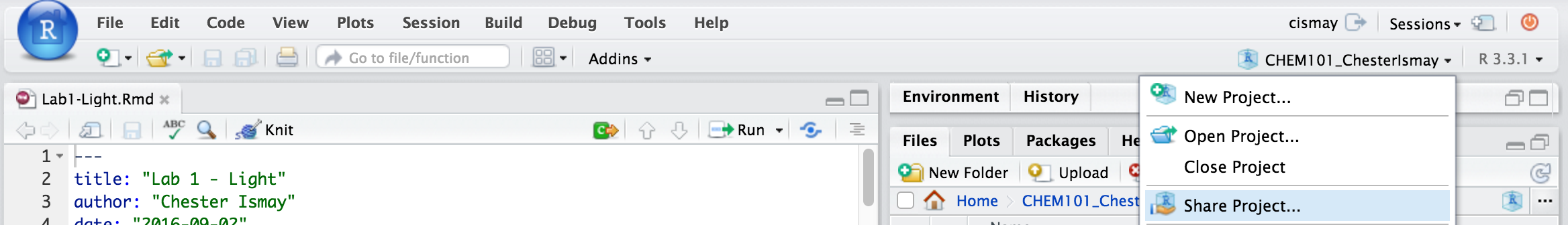
It is extremely helpful for us if you can share a link to your RStudio Project in any emails requesting help. This link is available by going to your RStudio project in the top right corner of RStudio, clicking on it and then selecting Share Project, and then select Sharing as seen in the screenshots below.

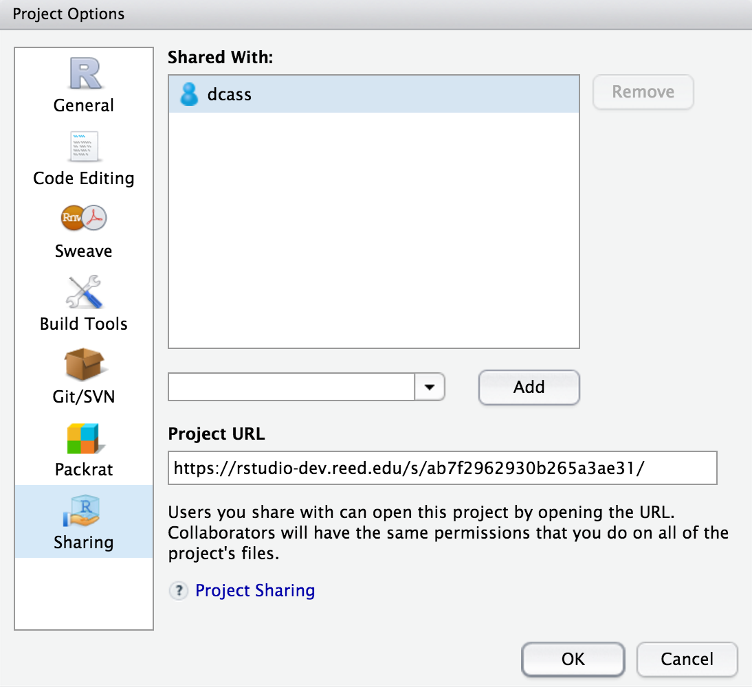
The link is given in the Project URL. Please copy this entire link into the body of your emails to Danielle or I so that we can quickly look into your errors.