Joining Techniques
📚 Schema reference · towns & counties 3 tables
- fips
- name
- state
- county_id
- county
- state
- fips_short
- county_seat
- county_seat_town_id
- year_established
- origin
- etymology
- population_2022
- land_area_sq_mi
- town_id
- town
- state
- primary_county
- secondary_county
- tertiary_county
- primary_county_id
- secondary_county_id
- tertiary_county_id
- population_2020_census
- population_2010_census
- land_area_sq_mi
Joins combine data from multiple tables. This is essential because real databases store related information in separate tables to avoid redundancy.
Reading the ERD: cardinality
Before joining two tables, read how their rows relate. On an entity relationship diagram (ERD), each end of a line says how many rows of that table one row of the other table can have. Two bars mean exactly one, a circle means zero is allowed, and the fan (a crow’s foot) means many. Scroll through three real relationships in this database.
One caution about this data: the Washington rows of pnw_towns are incomplete, so a few Washington counties show no towns or no county seat because rows are missing, not because the county has none. The diagrams point these out where they appear.
Cardinality: one county, many towns
pnw_towns.primary_county_id → pnw_counties.county_idScroll to build the diagram, one step at a time.
county_id of its county in primary_county_id, the foreign key. The colored chips are the same numbers on both sides. primary_county_id holds one value and is never NULL (0 of 453 towns). pnw_towns, whose Washington rows are incomplete; San Juan is the same. So this zero comes from incomplete data. The circle beside the crow's foot still belongs: it says the database allows a county with no towns, whatever the reason. That end reads zero or many. Text version of this diagram
- Step 1 · the tables. Four real counties and six real towns. Every town stores the
county_idof its county inprimary_county_id, the foreign key. The colored chips are the same numbers on both sides. - Step 2 · every town points once. Draw a line from each town to the county its chip matches. Every town gets exactly one line:
primary_county_idholds one value and is neverNULL(0 of 453 towns). - Step 3 · mark the county end. On an ERD, that fact goes at the county end of the line, because it answers "how many counties does one town have?" Two bars mean exactly one.
- Step 4 · count lines per county. Now look from the county side. Gilliam collects three lines, Harney two, Crook one. More than one is drawn as a crow's foot, the fan, at the town end.
- Step 5 · a county with no towns. Wahkiakum collects zero lines. It has towns in real life (its seat is Cathlamet), but none made it into
pnw_towns, whose Washington rows are incomplete; San Juan is the same. So this zero comes from incomplete data. The circle beside the crow's foot still belongs: it says the database allows a county with no towns, whatever the reason. That end reads zero or many. - Step 6 · read the whole line. Read each end as "one row of the other table has this many of me." One town has exactly one county; one county has zero or many towns (0 to 34 across all 75 in this data). That is a one-to-many relationship, and the foreign key sits on the many side.
Cardinality: zero or one, at both ends
pnw_counties.county_seat_town_id → pnw_towns.town_idScroll to build the diagram, one step at a time.
town_id of its seat in county_seat_town_id. Wahkiakum's seat, Cathlamet, is not in pnw_towns, so its value is NULL. town_id matches. A single column can hold only one value, so no county can draw two. pnw_towns, and Columbia County, Oregon lists "Saint Helens" where pnw_towns spells it "St. Helens", so the key was never filled in. Either way the database allows a county with zero or one seat town: a bar for "at most one", and a circle for "maybe none". Text version of this diagram
- Step 1 · the other key. The second line on the ERD runs the other way. Each county stores the
town_idof its seat incounty_seat_town_id. Wahkiakum's seat, Cathlamet, is not inpnw_towns, so its value isNULL. - Step 2 · counties point at their seat. Three counties draw one line each, to the town whose
town_idmatches. A single column can hold only one value, so no county can draw two. - Step 3 · the town end. Wahkiakum draws no line, like 5 of the 75 counties. Every county has a seat in real life, so these are data gaps: four seats (Friday Harbor, Cathlamet, Waterville, Coupeville) are missing from
pnw_towns, and Columbia County, Oregon lists "Saint Helens" wherepnw_townsspells it "St. Helens", so the key was never filled in. Either way the database allows a county with zero or one seat town: a bar for "at most one", and a circle for "maybe none". - Step 4 · the county end. From the town side: Burns, Condon, and Prineville are each the seat of exactly one county; Arlington, Hines, and Lonerock of none. Across the whole table no town is the seat of two counties.
- Step 5 · read the whole line. Zero or one at both ends: an optional one-to-one. Compare the first diagram, where the foreign key sat on the many side; here it sits on the county side, and the circles warn that a JOIN on it can come back empty.
Cardinality: many to many, and the bridge table
a town can lie in up to three counties; a county holds many townsScroll to build the diagram, one step at a time.
pnw_towns has three county keys: primary, secondary, and tertiary. Empty slots are NULL. primary_county_id alone gives the first diagram again: one solid line per town. town_id, county_id), which turns many-to-many into two one-to-many lines. This database stores the pairs as three columns instead, which caps a town at three counties and makes a query check all three. Text version of this diagram
- Step 1 · towns that straddle. 20 towns sit in more than one county, so
pnw_townshas three county keys: primary, secondary, and tertiary. Empty slots areNULL. - Step 2 · primary only. Using
primary_county_idalone gives the first diagram again: one solid line per town. - Step 3 · add the other keys. Add the secondary (dashed) and tertiary (dotted) keys. Albany now has 2 counties and Lake Oswego 3. One town, many counties.
- Step 4 · many on both sides. And one county still holds many towns: Linn collects Albany, Gates, and Idanha here (15 towns in all). Many at both ends is a many-to-many relationship.
- Step 5 · the bridge table. No single column can hold "many". The standard design is a bridge table with one row per line (
town_id,county_id), which turns many-to-many into two one-to-many lines. This database stores the pairs as three columns instead, which caps a town at three counties and makes a query check all three.
INNER JOIN
An INNER JOIN returns only rows where there’s a match in BOTH tables. Think of it as finding the intersection.
INNER JOIN: keep only matched rows
SELECT * FROM left_table AS l INNER JOIN right_table AS r ON l.id = r.id;Scroll to build the diagram, one step at a time.
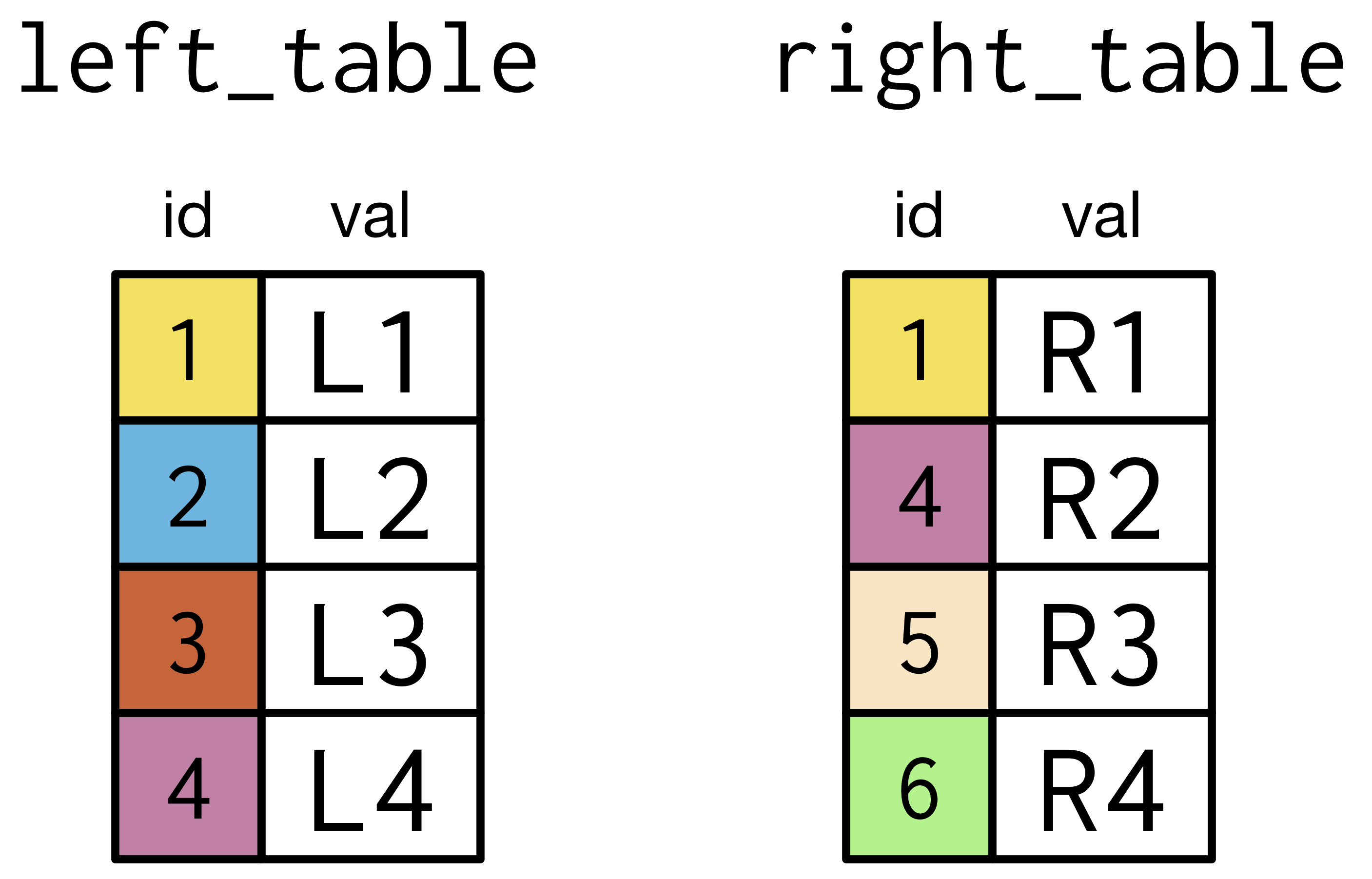
id key. Each key value has its own color so you can trace it. Keys 1 and 4 live in both; 2 and 3 are left-only; 5 and 6 are right-only. id column on both sides and asks one question of every value: does this key appear on the other side? val from each side. Text version of this diagram
- Step 1 · the tables. Two tables sharing an
idkey. Each key value has its own color so you can trace it. Keys 1 and 4 live in both; 2 and 3 are left-only; 5 and 6 are right-only. - Step 2 · the scan. An inner join walks the
idcolumn on both sides and asks one question of every value: does this key appear on the other side? - Step 3 · first match. Key 1 is in both tables, so the rows join and the first result row appears, carrying
valfrom each side. - Step 4 · second match. Key 4 matches too. The arrow crosses rows: position does not matter, only the key does.
- Step 5 · left rows with no match. Keys 2 and 3 look for a match on the right and find none (the open circles). An inner join drops them.
- Step 6 · right rows with no match. Keys 5 and 6 exist only on the right, so an inner join drops them as well. Unmatched on either side is gone.
- Step 7 · the result. Two tables in, two matched rows out. An inner join is the intersection: only keys on both sides survive.
Joining 1: Enrich town data with county information
Scenario: You want to see each town alongside when its county was established and the county’s etymology. This requires combining data from both tables. Show town, population_2020_census, county, year_established, and etymology (state isn’t selected here). Sort by population_2020_census, largest first.
Notice the join condition: pnw_towns.primary_county_id is a foreign key pointing at pnw_counties.county_id, so one equality is all it takes. Joining on names instead would need two conditions (t.primary_county = c.county AND t.state = c.state) — leave out the state and every town in Washington County, Oregon happily matches the state of Washington’s counties too. ID joins sidestep that trap entirely, which is why real warehouses key everything this way.
Joining 2: Find which towns are county seats
Scenario: County seats often have special administrative importance. Join to identify them. Show each seat’s town and state, its population as town_pop, its county, and the county’s population as county_pop. Sort by town_pop, largest first.
Joining 3: Compare town population to county population
Scenario: What percentage of each county’s population lives in each town? Show town, its population as town_pop, the county, its population as county_pop, and the percentage (1 decimal) as pct_of_county. Sort by pct_of_county, highest first.
LEFT JOIN
A LEFT JOIN returns ALL rows from the left table, plus matching rows from the right table. Non-matches get NULL values.
LEFT JOIN: keep every left row
SELECT * FROM left_table AS l LEFT JOIN right_table AS r ON l.id = r.id;Scroll to build the diagram, one step at a time.
val from both sides. NULL (the dark cells). NULL. A left join never loses a row from the left table, but it can hand you missing values to reckon with. Text version of this diagram
- Step 1 · the rule. Same two tables, new rule: keep every left row, matched or not. The left table is the one we protect.
- Step 2 · the matches. Keys 1 and 4 match as before, and their result rows come across complete with
valfrom both sides. - Step 3 · no match, but kept. Keys 2 and 3 find nothing on the right (open circles), but a left join keeps them anyway and fills the right columns with
NULL(the dark cells). - Step 4 · right rows with no match. Keys 5 and 6 exist only on the right. A left join does not keep extra right rows, so they are dropped.
- Step 5 · the result. Four rows out, one per left row, two of them carrying
NULL. A left join never loses a row from the left table, but it can hand you missing values to reckon with.
One thing to watch: if the right table has more than one row for a key, a matched left row is repeated once per match, so the join can return more rows than the left table started with.
One row, many matches: the join multiplies
-- right_dup has key 1 twice
SELECT * FROM left_table AS l LEFT JOIN right_dup AS r ON l.id = r.id;
Scroll to build the diagram, one step at a time.
R1 and R2). This is the case that quietly inflates row counts. NULL, exactly as a plain left join. L1 row double-counts. This is why you check the key is unique on the side you join to. Text version of this diagram
- Step 1 · a duplicated key. Here the right table has key 1 twice (
R1andR2). This is the case that quietly inflates row counts. - Step 2 · one-to-many. Left key 1 matches both right rows, so it produces two result rows. One left row became two: the join multiplied it.
- Step 3 · the other match. Key 4 matches a single right row, so it stays one row. Only the duplicated key multiplied.
- Step 4 · no match, but kept. Keys 2 and 3 still have no match and are kept with
NULL, exactly as a plain left join. - Step 5 · the result. Five rows out from four left rows. If you were counting or summing, that extra
L1row double-counts. This is why you check the key is unique on the side you join to.
Joining 4: List all counties with their county seat populations (if available)
Scenario: Some county seats might not be in our towns database. LEFT JOIN ensures all counties appear. Show county, state, county_seat, and the seat’s population as seat_population. List counties with no seat_population first, then sort alphabetically by county.
Joining 5: Flag whether each town is a county seat
Scenario: Add a column indicating county seat status for every town. Show town, state, population_2020_census, an is_county_seat flag of ‘Yes’ or ‘No’, and the county served as seat_of_county. List county seats first, then sort by population_2020_census, largest first.
Anti-Join
An anti-join finds rows in one table that have NO match in another table. It’s implemented as a LEFT JOIN with a WHERE clause checking for NULLs.
Anti-join: keep only the left rows with no match
SELECT l.* FROM left_table AS l
 LEFT JOIN right_table AS r ON l.id = r.id
 WHERE r.id IS NULL;
Scroll to build the diagram, one step at a time.
NULL. WHERE r.id IS NULL filter keeps only the rows whose right side never matched. The matched rows drop out, and you are left with the left-only keys 2 and 3. Text version of this diagram
- Step 1 · start from a left join. An anti-join is a left join with a twist. First, line up the two tables the same way.
- Step 2 · the matches. Keys 1 and 4 match on the right. These are exactly the rows an anti-join wants to throw away.
- Step 3 · the non-matches. Keys 2 and 3 have no match on the right (open circles). After a left join, their right columns are
NULL. - Step 4 · WHERE r.id IS NULL. The
WHERE r.id IS NULLfilter keeps only the rows whose right side never matched. The matched rows drop out, and you are left with the left-only keys 2 and 3.
Joining 6: Find county seats not in our towns database
Scenario: Data quality check - which county seats are missing from our towns table? List each affected county with its state and county_seat. Sort by state, then alphabetically by county.
Joining 7: Find large towns that are NOT county seats
Scenario: Identify towns with more than 25,000 people that are not county seats. Show town, state, population_2020_census, and primary_county. Sort by population_2020_census, largest first.
Joining 8: Find counties with no towns in our database
Scenario: Which counties have zero incorporated towns listed? This might indicate missing data. Show each such county with its state, population_2022, and county_seat. Sort by population_2022, largest first.
Order of operations: putting it together
A query with a join, a filter, groups, a sort, and a LIMIT does not run in the order it is written. The first diagram lines the two orders up; the second runs one real query through all eight clauses, from FROM to LIMIT. (The single-table version is on Sorting and Grouping.)
Written order vs. the order SQL runs it
SELECT …
  FROM … JOIN … ON …
 WHERE …
 GROUP BY …
HAVING …
 ORDER BY …
 LIMIT …;
Scroll to build the diagram, one step at a time.
SELECT first, then FROM and any JOIN, then the filters, and LIMIT last. FROM and JOIN … ON come first. FROM, JOIN, WHERE, GROUP BY, and HAVING each move up only one slot, and ORDER BY and LIMIT stay at the end. SELECT is typed first but runs sixth. By the time it runs, the join is done, rows are filtered, and groups are formed. That is why, in standard SQL, a column alias such as AS pop works in ORDER BY but not in WHERE or HAVING. SQLite, which runs this site, lets an alias slide in those clauses, but PostgreSQL and SQL Server reject it, so repeat the expression to keep a query working everywhere. LIMIT. The next diagram runs one real query through all eight. Text version of this diagram
- Step 1 · the order you type. Every query on this site is written in this order:
SELECTfirst, thenFROMand anyJOIN, then the filters, andLIMITlast. - Step 2 · the order SQL runs. SQL runs the same clauses in a different order. It needs rows before it can do anything else, so
FROMandJOIN … ONcome first. - Step 3 · most clauses keep their place.
FROM,JOIN,WHERE,GROUP BY, andHAVINGeach move up only one slot, andORDER BYandLIMITstay at the end. - Step 4 · SELECT is the one that moves.
SELECTis typed first but runs sixth. By the time it runs, the join is done, rows are filtered, and groups are formed. That is why, in standard SQL, a column alias such asAS popworks inORDER BYbut not inWHEREorHAVING. SQLite, which runs this site, lets an alias slide in those clauses, but PostgreSQL and SQL Server reject it, so repeat the expression to keep a query working everywhere. - Step 5 · two halves. Read the run order in two halves. Steps 1 to 5 build and filter rows. Steps 6 to 8 shape the output: pick the columns, sort them, and keep the first few with
LIMIT. The next diagram runs one real query through all eight.
One join query, run clause by clause
SELECT c.county, COUNT(*) AS n_towns,
       SUM(t.population_2020_census) AS pop
  FROM pnw_towns AS t
  JOIN pnw_counties AS c
    ON c.county_id = t.primary_county_id
 WHERE c.state = 'Oregon'
   AND c.county IN ('Crook', 'Harney', 'Jefferson')
 GROUP BY c.county
HAVING COUNT(*) >= 2
 ORDER BY pop DESC
 LIMIT 1;
Scroll to build the diagram, one step at a time.
FROM pnw_towns AS t: all 453 towns. Eight are shown here; the other rows go through the same steps. t.pop is short for t.population_2020_census. JOIN … ON runs next. Each town's primary_county_id is matched to a county_id, and the town's row gains that county's columns: Prineville gets Crook, Bend gets Deschutes. The join is finished before any filter runs. WHERE filters the joined rows, so it can test county columns. Bend is out (Deschutes). So is Port Townsend: Washington has a Jefferson County too, and c.state = 'Oregon' is the only thing that excludes it. Six rows are left. GROUP BY c.county sorts the six rows into three groups: Crook (1 town), Harney (2), and Jefferson (3). COUNT(*) and SUM. HAVING COUNT(*) >= 2 filters groups, so Crook, with one town, drops out. WHERE could not do this: the counts did not exist yet when it ran. SELECT run. It names the output columns and creates the aliases n_towns and pop. In standard SQL nothing earlier can use those names, because they did not exist yet. SQLite, which runs this site, would accept HAVING n_towns >= 2 anyway; writing HAVING COUNT(*) >= 2 keeps the query working in PostgreSQL and SQL Server too. ORDER BY pop DESC sorts the finished rows, and it can use the alias pop because SELECT has already run. Jefferson (10,036) moves ahead of Harney (4,375). LIMIT 1 runs last and keeps only the first row of the sorted result: Jefferson, 3 towns, 10,036 people. Because it runs after ORDER BY, LIMIT keeps the top rows of the sort; without an ORDER BY, which rows you get is not guaranteed. Text version of this diagram
- Step 1 · FROM. SQL starts with
FROM pnw_towns AS t: all 453 towns. Eight are shown here; the other rows go through the same steps.t.popis short fort.population_2020_census. - Step 2 · JOIN … ON.
JOIN … ONruns next. Each town'sprimary_county_idis matched to acounty_id, and the town's row gains that county's columns: Prineville gets Crook, Bend gets Deschutes. The join is finished before any filter runs. - Step 3 · WHERE.
WHEREfilters the joined rows, so it can test county columns. Bend is out (Deschutes). So is Port Townsend: Washington has a Jefferson County too, andc.state = 'Oregon'is the only thing that excludes it. Six rows are left. - Step 4 · GROUP BY.
GROUP BY c.countysorts the six rows into three groups: Crook (1 town), Harney (2), and Jefferson (3). - Step 5 · HAVING. Each group is now one row, with its
COUNT(*)andSUM.HAVING COUNT(*) >= 2filters groups, so Crook, with one town, drops out.WHEREcould not do this: the counts did not exist yet when it ran. - Step 6 · SELECT. Only now does
SELECTrun. It names the output columns and creates the aliasesn_townsandpop. In standard SQL nothing earlier can use those names, because they did not exist yet. SQLite, which runs this site, would acceptHAVING n_towns >= 2anyway; writingHAVING COUNT(*) >= 2keeps the query working in PostgreSQL and SQL Server too. - Step 7 · ORDER BY.
ORDER BY pop DESCsorts the finished rows, and it can use the aliaspopbecauseSELECThas already run. Jefferson (10,036) moves ahead of Harney (4,375). - Step 8 · LIMIT.
LIMIT 1runs last and keeps only the first row of the sorted result: Jefferson, 3 towns, 10,036 people. Because it runs afterORDER BY,LIMITkeeps the top rows of the sort; without anORDER BY, which rows you get is not guaranteed.
Going further
Two more join examples combine a join with GROUP BY: counting towns per county (including the counties with none) and a full county dashboard. They are in Going Further.