Statistical Inference: A Tidy Approach

# Statistical Inference: A Tidy Approach
### Dr. Chester Ismay Senior Curriculum Lead at <a href="https://www.datacamp.com/">DataCamp</a> <a href="http://github.com/ismayc">  ismayc</a> <a href="http://twitter.com/old_man_chester">   @old_man_chester</a> <a href="mailto:chester@datacamp.com">  chester@datacamp.com</a> 
### 2018-04-13 New England Statistical Symposium - UMass Amherst Slides available at <a href="http://bit.ly/ness-infer" class="uri">http://bit.ly/ness-infer</a> PDF slides at <a href="http://bit.ly/ness-infer-pdf" class="uri">http://bit.ly/ness-infer-pdf</a>

---

# Table of Contents

Part 1
- [Data Wrangling](#wrangling)
- [Data Visualization](#viz)
- [Data Tidying](#tidying)

Part 2
- [Resampling](#resampling)
- [Inference](#inference)

.footer[R code from throughout the slides is saved as an R script [here](https://raw.githubusercontent.com/ismayc/talks/master/ness-infer/slide_code.R)]
---

.footer[Slides available at http://bit.ly/ness-infer &emsp; &emsp; &emsp; [Return to Table of Contents](#toc)]

---

## Prior Installation

Make sure you have the (current) up-to-date R, RStudio, and R packages
- [Beginner's Guide](http://moderndive.com/2-getting-started.html) on ModernDive.com

***

- [R (version 3.4.4)](https://cran.r-project.org/)
- [RStudio (version 1.1.442)](https://www.rstudio.com/products/rstudio/download3/)

- Run this in the RStudio Console

```r
pkgs <- c("tidyverse", "moderndive", "gapminder",
 "nycflights13", "fivethirtyeight", "janitor",
 "ggplot2movies", "remotes")

install.packages(pkgs)
remotes::install_github("andrewpbray/infer")
```

---

## Freely available information

<center><h2>A Modern Dive into Data with R</h2></center>

* Webpage: <http://moderndive.com>
* Developmental version at <https://moderndive.netlify.com>
* [GitHub Repo](https://github.com/moderndive/moderndiver-book)
* Please [signup](http://eepurl.com/cBkItf) for our mailing list!

---

---

.footer[Slides available at http://bit.ly/ness-infer &emsp; &emsp; &emsp; [Return to Table of Contents](#toc)]

---

## Designed for the novice / Nice for the practioner

---

## Designed for the novice / Nice for the practioner

---

# R Data Types

---

## The bare minimum needed for understanding today

Vector/variable
  - Type of vector (`int`, `num` or `dbl`, `chr`, `lgl`, `date`)

Data frame
  - Vectors of (potentially) different types
  - Each vector has the same number of rows

---

## The bare minimum needed for understanding today

```r
library(tibble)
library(lubridate)
ex1 <- data_frame(
 vec1 = c(1980, 1990, 2000, 2010),
 vec2 = c(1L, 2L, 3L, 4L),
 vec3 = c("low", "low", "high", "high"),
 vec4 = c(TRUE, FALSE, FALSE, FALSE),
 vec5 = ymd(c("2017-05-23", "1776/07/04", 
 "1983-05/31", "1908/04-01"))
 )
ex1
```

```
# A tibble: 4 x 5
 vec1 vec2 vec3 vec4 vec5 
 <dbl> <int> <chr> <lgl> <date> 
1 1980. 1 low TRUE 2017-05-23
2 1990. 2 low FALSE 1776-07-04
3 2000. 3 high FALSE 1983-05-31
4 2010. 4 high FALSE 1908-04-01
```
 
---

class: center, middle 
 
# Welcome to the [tidyverse](https://blog.rstudio.org/2016/09/15/tidyverse-1-0-0/)!
 
The `tidyverse` is a collection of R packages that share common philosophies and are designed to work together. 
 
<a href="http://tidyverse.tidyverse.org/logo.png"><img src="figure/tidyverse.png" style="width: 200px;"/></a>

---

# First motivating example for today

- Inspired by the late, great [Hans Rosling](https://www.youtube.com/watch?v=jbkSRLYSojo)

---

# Data Wrangling

---

.footer[Slides available at http://bit.ly/ness-infer &emsp; &emsp; &emsp; [Return to Table of Contents](#toc)]

---

## The [`gapminder` package](https://github.com/jennybc/gapminder)

```r
library(gapminder)
gapminder
```

```
# A tibble: 1,704 x 6
 country continent year lifeExp pop gdpPercap
 <fct> <fct> <int> <dbl> <int> <dbl>
 1 Afghanistan Asia 1952 28.8 8425333 779.
 2 Afghanistan Asia 1957 30.3 9240934 821.
 3 Afghanistan Asia 1962 32.0 10267083 853.
 4 Afghanistan Asia 1967 34.0 11537966 836.
 5 Afghanistan Asia 1972 36.1 13079460 740.
 6 Afghanistan Asia 1977 38.4 14880372 786.
 7 Afghanistan Asia 1982 39.9 12881816 978.
 8 Afghanistan Asia 1987 40.8 13867957 852.
 9 Afghanistan Asia 1992 41.7 16317921 649.
10 Afghanistan Asia 1997 41.8 22227415 635.
# ... with 1,694 more rows
```

---

## Base R versus the `tidyverse`

- The mean life expectancy across all years for Asia
--

```r
# Base R
asia <- gapminder[gapminder$continent == "Asia", ]
mean(asia$lifeExp)
```

```
[1] 60.065
```
--

```r
library(dplyr)
gapminder %>% filter(continent == "Asia") %>%
  summarize(mean_exp = mean(lifeExp))
```

```
[1] 60.065
```

---

## The pipe `%>%`

<img src="figure/pipe.png" style="width: 240px;"/> &emsp; &emsp; &emsp; <img src="figure/MagrittePipe.jpg" style="width: 300px;"/>
--

- A way to chain together commands
- Can be read as "and then" when reading over code
--

```r
library(dplyr)
gapminder %>% filter(continent == "Asia") %>%
  summarize(mean_exp = mean(lifeExp))
```

---

# [The Five Main Verbs (5MV)](http://moderndive.com/5-wrangling.html) of data wrangling

- [`filter()`](#filter) 
- [`summarize()`](#summarize)
- [`group_by()`](#groupby)
- [`mutate()`](#mutate) 
- [`arrange()`](#arrange)

---

## `filter()`

- Select a subset of the rows of a data frame.

- Arguments are "filters" that you'd like to apply.
--

```r
library(gapminder); library(dplyr)
gap_2007 <- gapminder %>% filter(year == 2007)
head(gap_2007, 4)
```

```
# A tibble: 4 x 6
 country continent year lifeExp pop gdpPercap
 <fct> <fct> <int> <dbl> <int> <dbl>
1 Afghanistan Asia 2007 43.8 31889923 975.
2 Albania Europe 2007 76.4 3600523 5937.
3 Algeria Africa 2007 72.3 33333216 6223.
4 Angola Africa 2007 42.7 12420476 4797.
```

- Use `==` to compare a variable to a value

---

## Logical operators

- Use `|` to check for any in multiple filters being true:
--

```r
gapminder %>% 
  filter(year == 2002 | continent == "Asia") %>% 
  sample_n(8)
```
--

```
# A tibble: 8 x 6
 country continent year lifeExp pop gdpPercap
 <fct> <fct> <int> <dbl> <int> <dbl>
1 Iraq Asia 1997 58.8 20775703 3076.
2 Korea, Rep. Asia 1997 74.6 46173816 15994.
3 Bangladesh Asia 1952 37.5 46886859 684.
4 France Europe 2002 79.6 59925035 28926.
5 Kuwait Asia 1957 58.0 212846 113523.
6 Iran Asia 1962 49.3 22874000 4187.
7 Myanmar Asia 1982 58.1 34680442 424.
8 Canada Americas 2002 79.8 31902268 33329.
```

---

## Logical operators

- Use `,` to check for all of multiple filters being true:
--

```r
gapminder %>% 
  filter(year == 2002, continent == "Asia")
```

```
# A tibble: 8 x 6
 country continent year lifeExp pop gdpPercap
 <fct> <fct> <int> <dbl> <int> <dbl>
1 Afghanistan Asia 2002 42.1 25268405 727.
2 Bahrain Asia 2002 74.8 656397 23404.
3 Bangladesh Asia 2002 62.0 135656790 1136.
4 Cambodia Asia 2002 56.8 12926707 896.
5 China Asia 2002 72.0 1280400000 3119.
6 Hong Kong, China Asia 2002 81.5 6762476 30209.
7 India Asia 2002 62.9 1034172547 1747.
8 Indonesia Asia 2002 68.6 211060000 2874.
```

---

## Logical operators

- Use `%in%` to check for any being true (shortcut to using `|` repeatedly with `==`)
--

```r
gapminder %>% 
  filter(country %in% c("Argentina", "Belgium", "Mexico"),
         year %in% c(1987, 1992))
```
--

```
# A tibble: 6 x 6
 country continent year lifeExp pop gdpPercap
 <fct> <fct> <int> <dbl> <int> <dbl>
1 Argentina Americas 1987 70.8 31620918 9140.
2 Argentina Americas 1992 71.9 33958947 9308.
3 Belgium Europe 1987 75.4 9870200 22526.
4 Belgium Europe 1992 76.5 10045622 25576.
5 Mexico Americas 1987 69.5 80122492 8688.
6 Mexico Americas 1992 71.5 88111030 9472.
```

---

## `summarize()`

- Any numerical summary that you want to apply to a column of a data frame is specified within `summarize()`.

```r
stats_1997 <- gapminder %>% 
 filter(year == 1997) %>% 
 summarize(max_exp = max(lifeExp),
 sd_exp = sd(lifeExp))
stats_1997
```
--

```
# A tibble: 1 x 2
 max_exp sd_exp
 <dbl> <dbl>
1 80.7 11.6
```

---

### Combining `summarize()` with `group_by()`

When you'd like to determine a numerical summary for all
levels of a different categorical variable

```r
max_exp_1997_by_cont <- gapminder %>% 
 filter(year == 1997) %>% 
 group_by(continent) %>%
 summarize(max_exp = max(lifeExp),
 sd_exp = sd(lifeExp))
max_exp_1997_by_cont
```

```
# A tibble: 5 x 3
 continent max_exp sd_exp
 <fct> <dbl> <dbl>
1 Africa 74.8 9.10 
2 Americas 78.6 4.89 
3 Asia 80.7 8.09 
4 Europe 79.4 3.10 
5 Oceania 78.8 0.905
```

---

## `mutate()`

- Allows you to 
 1. create a new variable with a specific value OR
 2. create a new variable based on other variables OR
 3. change the contents of an existing variable

```r
gap_plus <- gapminder %>% mutate(just_one = 1)
head(gap_plus, 4)
```

```
# A tibble: 4 x 7
 country continent year lifeExp pop gdpPercap just_one
 <fct> <fct> <int> <dbl> <int> <dbl> <dbl>
1 Afghanistan Asia 1952 28.8 8425333 779. 1.
2 Afghanistan Asia 1957 30.3 9240934 821. 1.
3 Afghanistan Asia 1962 32.0 10267083 853. 1.
4 Afghanistan Asia 1967 34.0 11537966 836. 1.
```

---

## `mutate()`

- Allows you to 
 1. create a new variable with a specific value OR
 2. create a new variable based on other variables OR
 3. change the contents of an existing variable

```r
gap_w_gdp <- gapminder %>% mutate(gdp = pop * gdpPercap)
sample_n(gap_w_gdp, 4)
```

```
# A tibble: 4 x 7
 country continent year lifeExp pop gdpPercap gdp
 <fct> <fct> <int> <dbl> <int> <dbl> <dbl>
1 Comoros Africa 1967 46.5 217378 1876. 407807572.
2 Paraguay Americas 1992 68.2 4483945 4196. 18816476471.
3 Mauritius Africa 1967 61.6 789309 2475. 1953845681.
4 Chile Americas 1997 75.8 14599929 10118. 147722858046.
```

---

## `mutate()`

- Allows you to 
 1. create a new variable with a specific value OR
 2. create a new variable based on other variables OR
 3. change the contents of an existing variable

```r
gap_weird <- gapminder %>% mutate(pop = pop + 1000)
head(gap_weird, 4)
```

```
# A tibble: 4 x 6
 country continent year lifeExp pop gdpPercap
 <fct> <fct> <int> <dbl> <dbl> <dbl>
1 Afghanistan Asia 1952 28.8 8426333. 779.
2 Afghanistan Asia 1957 30.3 9241934. 821.
3 Afghanistan Asia 1962 32.0 10268083. 853.
4 Afghanistan Asia 1967 34.0 11538966. 836.
```

---

## `arrange()`

- Reorders the rows in a data frame based on the values of one or more variables
--

```r
gapminder %>% arrange(year, country) %>% head(10)
```

```
# A tibble: 10 x 6
 country continent year lifeExp pop gdpPercap
 <fct> <fct> <int> <dbl> <int> <dbl>
 1 Afghanistan Asia 1952 28.8 8425333 779.
 2 Albania Europe 1952 55.2 1282697 1601.
 3 Algeria Africa 1952 43.1 9279525 2449.
 4 Angola Africa 1952 30.0 4232095 3521.
 5 Argentina Americas 1952 62.5 17876956 5911.
 6 Australia Oceania 1952 69.1 8691212 10040.
 7 Austria Europe 1952 66.8 6927772 6137.
 8 Bahrain Asia 1952 50.9 120447 9867.
 9 Bangladesh Asia 1952 37.5 46886859 684.
10 Belgium Europe 1952 68.0 8730405 8343.
```

---

## `arrange()`

- Can also put into descending order
--

```r
gapminder %>%
  filter(year > 2000) %>%
  arrange(desc(lifeExp)) %>%
  head(10)
```

```
# A tibble: 10 x 6
 country continent year lifeExp pop gdpPercap
 <fct> <fct> <int> <dbl> <int> <dbl>
 1 Japan Asia 2007 82.6 127467972 31656.
 2 Hong Kong, China Asia 2007 82.2 6980412 39725.
 3 Japan Asia 2002 82.0 127065841 28605.
 4 Iceland Europe 2007 81.8 301931 36181.
 5 Switzerland Europe 2007 81.7 7554661 37506.
 6 Hong Kong, China Asia 2002 81.5 6762476 30209.
 7 Australia Oceania 2007 81.2 20434176 34435.
 8 Spain Europe 2007 80.9 40448191 28821.
 9 Sweden Europe 2007 80.9 9031088 33860.
10 Israel Asia 2007 80.7 6426679 25523.
```

---

## Don't mix up `arrange` and `group_by`

- `group_by` is used (mostly) with `summarize` to calculate summaries over groups

- `arrange` is used for sorting

---

## Don't mix up `arrange` and `group_by`

This doesn't really do anything useful

```r
gapminder %>% group_by(year)
```

```
# A tibble: 1,704 x 6
# Groups: year [12]
 country continent year lifeExp pop gdpPercap
 <fct> <fct> <int> <dbl> <int> <dbl>
 1 Afghanistan Asia 1952 28.8 8425333 779.
 2 Afghanistan Asia 1957 30.3 9240934 821.
 3 Afghanistan Asia 1962 32.0 10267083 853.
 4 Afghanistan Asia 1967 34.0 11537966 836.
 5 Afghanistan Asia 1972 36.1 13079460 740.
 6 Afghanistan Asia 1977 38.4 14880372 786.
 7 Afghanistan Asia 1982 39.9 12881816 978.
 8 Afghanistan Asia 1987 40.8 13867957 852.
 9 Afghanistan Asia 1992 41.7 16317921 649.
10 Afghanistan Asia 1997 41.8 22227415 635.
# ... with 1,694 more rows
```

---

## Don't mix up `arrange` and `group_by`

But this does

```r
gapminder %>% arrange(year)
```

```
# A tibble: 1,704 x 6
 country continent year lifeExp pop gdpPercap
 <fct> <fct> <int> <dbl> <int> <dbl>
 1 Afghanistan Asia 1952 28.8 8425333 779.
 2 Albania Europe 1952 55.2 1282697 1601.
 3 Algeria Africa 1952 43.1 9279525 2449.
 4 Angola Africa 1952 30.0 4232095 3521.
 5 Argentina Americas 1952 62.5 17876956 5911.
 6 Australia Oceania 1952 69.1 8691212 10040.
 7 Austria Europe 1952 66.8 6927772 6137.
 8 Bahrain Asia 1952 50.9 120447 9867.
 9 Bangladesh Asia 1952 37.5 46886859 684.
10 Belgium Europe 1952 68.0 8730405 8343.
# ... with 1,694 more rows
```

---

## Practice

Use the [5MV](#fivemv) to answer problems from R data packages, e.g., [`nycflights13::weather`]

1. What is the maximum arrival delay for each carrier departing JFK? [`nycflights13::flights`]

2. Calculate for each movie the domestic return on investment for 2013 scaled data descending by ROI [`fivethirtyeight::bechdel`]

---

# Data Visualization

<center>
<a href="https://ggplot2.tidyverse.org">
<img src="img/ggplot2_hex.png" style = "width: 400px;"/>
</a>
</center>
---

.footer[Slides available at http://bit.ly/ness-infer &emsp; &emsp; &emsp; [Return to Table of Contents](#toc)]

---
<img src="slide_deck_files/figure-html/unnamed-chunk-29-1.png" style="display: block; margin: auto;" />

- What are the variables here?
- What is the observational unit?
- How are the variables mapped to aesthetics?

---

## Grammar of Graphics

Wilkinson (2005) laid out the proposed "Grammar of Graphics"

---

## Grammar of Graphics in R

Wickham implemented the grammar in R in the `ggplot2` package

---

## What is a statistical graphic?

## A `mapping` of `data` variables

## to `aes()`thetic attributes

## of `geom_`etric objects.

---

# Back to Basics

---

## Old school

- Sketch the graphics below on paper, where the `x`-axis is variable `A` and the `y`-axis is variable `B`

```
# A tibble: 4 x 4
 A B C D 
 <dbl> <dbl> <dbl> <chr>
1 1980. 1. 3. cold 
2 1990. 2. 2. cold 
3 2000. 3. 1. hot 
4 2010. 4. 2. hot 
```

1. A scatter plot
1. A scatter plot where the `color` of the points corresponds to `D`
1. A scatter plot where the `size` of the points corresponds to `C`

---

.footer[Slides available at http://bit.ly/ness-infer &emsp; &emsp; &emsp; [Return to Table of Contents](#toc)]

---

## Reproducing the plots in `ggplot2`

### 1. A scatterplot

```r
library(ggplot2)
ggplot(data = simple_ex, mapping = aes(x = A, y = B)) + 
  geom_point()
```
--

![](slide_deck_files/figure-html/unnamed-chunk-32-1.png)

---

## Reproducing the plots in `ggplot2`

### 2. A scatter plot where the `color` of the points corresponds to `D`

```r
library(ggplot2)
ggplot(data = simple_ex, mapping = aes(x = A, y = B)) + 
  geom_point(mapping = aes(color = D))
```
--

![](slide_deck_files/figure-html/unnamed-chunk-34-1.png)

---

## Reproducing the plots in `ggplot2`

### 3. A scatter plot where the `size` of the points corresponds to `C`

```r
library(ggplot2)
ggplot(data = simple_ex, mapping = aes(x = A, y = B, size = C)) + 
  geom_point()
```
--

![](slide_deck_files/figure-html/unnamed-chunk-36-1.png)

---

# [The Five-Named Graphs](http://moderndive.com/3-viz.html#FiveNG)

## The 5NG of data viz

- Scatterplot: `geom_point()`
- Line graph: `geom_line()`
- Histogram: `geom_histogram()`
- Boxplot: `geom_boxplot()`
- Bar graph: `geom_bar()`

---

## More examples

---

## Histogram

```r
library(nycflights13)
ggplot(data = weather, mapping = aes(x = humid)) +
  geom_histogram(bins = 20, color = "black", fill = "darkorange")
```

![](slide_deck_files/figure-html/unnamed-chunk-37-1.png)

---

## Boxplot (broken)

```r
library(nycflights13)
ggplot(data = weather, mapping = aes(x = month, y = humid)) +
  geom_boxplot()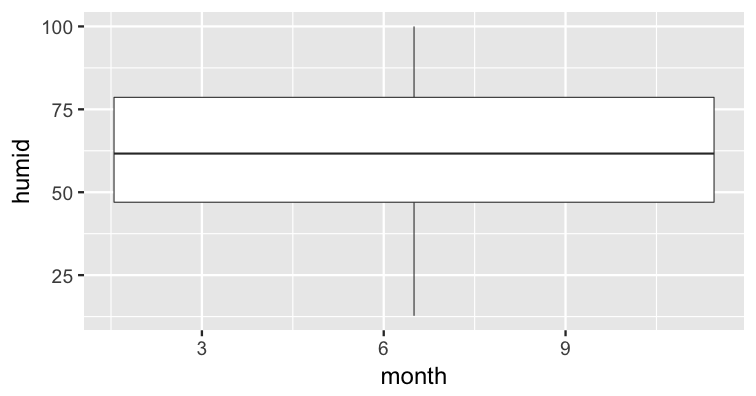
```

![](slide_deck_files/figure-html/unnamed-chunk-38-1.png)

---

## Boxplot (fixed)

```r
library(nycflights13)
ggplot(data = weather, mapping = aes(x = factor(month), y = humid)) +
  geom_boxplot()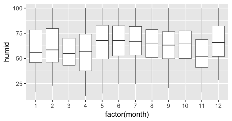
```

![](slide_deck_files/figure-html/unnamed-chunk-39-1.png)

---

## Bar graph

```r
library(fivethirtyeight)
ggplot(data = bechdel, mapping = aes(x = clean_test)) +
  geom_bar()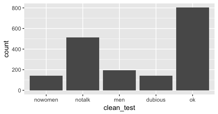
```

![](slide_deck_files/figure-html/unnamed-chunk-40-1.png)

---

## How about over time?

- One more variable to create with `dplyr`

```r
library(dplyr)
year_bins <- c("'70-'74", "'75-'79", "'80-'84", "'85-'89",
 "'90-'94", "'95-'99", "'00-'04", "'05-'09",
 "'10-'13")
bechdel <- bechdel %>%
 mutate(five_year = cut(year, 
 breaks = seq(1969, 2014, 5), 
 labels = year_bins))
```

---

## How about over time? (Stacked)

```r
library(fivethirtyeight)
library(ggplot2)
ggplot(data = bechdel,
       mapping = aes(x = five_year, fill = clean_test)) +
  geom_bar() +
  scale_fill_brewer(type = "qual") # set colors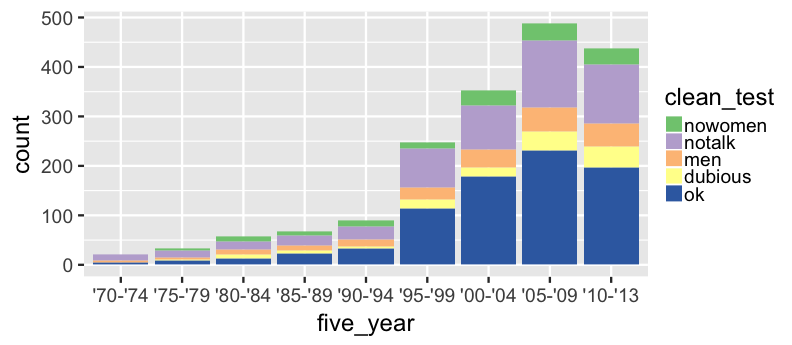
```

![](slide_deck_files/figure-html/unnamed-chunk-42-1.png)

---

## How about over time? (Side-by-side)

```r
library(fivethirtyeight)
library(ggplot2)
ggplot(data = bechdel,
       mapping = aes(x = five_year, fill = clean_test)) +
  geom_bar(position = "dodge") +
  scale_fill_brewer(type = "qual")
```

![](slide_deck_files/figure-html/unnamed-chunk-43-1.png)

---

## How about over time? (Stacked proportional)

```r
library(fivethirtyeight)
library(ggplot2)
ggplot(data = bechdel,
       mapping = aes(x = five_year, fill = clean_test)) +
  geom_bar(position = "fill", color = "black") +
  scale_fill_brewer(type = "qual")
```

![](slide_deck_files/figure-html/unnamed-chunk-44-1.png)

---

## `ggplot2` is for beginners and for data science professionals!

---

## Practice

Produce appropriate 5NG with R package & data set in [ ], e.g., [`nycflights13::weather`]

1. How does `age` predict `recline_rude`? [`fivethirtyeight::flying`]

2. Distribution of log base 10 scale of `budget_2013` [`fivethirtyeight::bechdel`]

3. How does `budget` predict `rating`? [`ggplot2movies::movies`]

---

### HINTS

![](slide_deck_files/figure-html/unnamed-chunk-45-1.png)

---

# DEMO in RStudio

---

### Determining the appropriate plot

---

# Data Tidying

---

.footer[Slides available at http://bit.ly/ness-infer &emsp; &emsp; &emsp; [Return to Table of Contents](#toc)]

---

# Tidy Data?

1. Each variable forms a column.
2. Each observation forms a row.
3. Each type of observational unit forms a table.

The third point means we don't mix apples and oranges.

---

## What is Tidy Data?

1. Each observation forms a row. In other words, each row corresponds to a single instance of an observational unit
1. Each variable forms a column:
 + Some variables may be used to identify the observational units. 
 + For organizational purposes, it's generally better to put these in the left-hand columns
1. Each type of observational unit forms a table.

---

## Differentiating between neat data and tidy data

- Colloquially, they mean the same thing
- But in our context, one is a subset of the other.

Neat data is 
 - easy to look at, 
 - organized nicely, and 
 - in table form.

Tidy data is neat but also abides by a set of three rules.

---

---

## Is this tidy?

```
# A tibble: 12 x 4
 year title clean_test budget_2013
 <int> <chr> <ord> <int>
 1 1995 Apollo 13 ok 99370665
 2 2005 Brokeback Mountain notalk 16583160
 3 2010 Diary of a Wimpy Kid ok 16023478
 4 1984 Dune dubious 100864980
 5 1984 Ghostbusters notalk 67243320
 6 2003 How to Lose a Guy in 10 Days men 63304348
 7 2011 Iris ok 5696299
 8 2004 Sideways ok 20964279
 9 2000 Songcatcher ok 2435235
10 2004 Team America: World Police men 24663858
11 2010 Tron Legacy notalk 213646368
12 2011 War Horse notalk 72498355
```

---

## How about this? Is this tidy?

```
# A tibble: 12 x 13
 country `1952` `1957` `1962` `1967` `1972` `1977` `1982` `1987`
 <chr> <int> <int> <int> <int> <int> <int> <int> <int>
 1 Albania -9 -9 -9 -9 -9 -9 -9 -9
 2 Argentina -9 -1 -1 -9 -9 -9 -8 8
 3 Armenia -9 -7 -7 -7 -7 -7 -7 -7
 4 Australia 10 10 10 10 10 10 10 10
 5 Austria 10 10 10 10 10 10 10 10
 6 Azerbaijan -9 -7 -7 -7 -7 -7 -7 -7
 7 Belarus -9 -7 -7 -7 -7 -7 -7 -7
 8 Belgium 10 10 10 10 10 10 10 10
 9 Bhutan -10 -10 -10 -10 -10 -10 -10 -10
10 Bolivia -4 -3 -3 -4 -7 -7 8 9
11 Brazil 5 5 5 -9 -9 -4 -3 7
12 Bulgaria -7 -7 -7 -7 -7 -7 -7 -7
# ... with 4 more variables: `1992` <int>, `1997` <int>,
# `2002` <int>, `2007` <int>
```

---

## Why is tidy data important?

- Think about trying to plot democracy score across years in the simplest way possible with the data on the [previous slide](#demscore).
--

- It would be much easier if the data looked like what follows instead so we could put 
    - `year` on the `x`-axis and 
    - `dem_score` on the `y`-axis.

---

## Tidy is good

```r
library(tidyr)
dem_score_tidy <- dem_score %>% 
 gather(-country, key = "year", value = "dem_score") %>% 
 mutate(year = as.integer(year)) 
dem_score_tidy %>% sample_n(10) %>% arrange(country)
```
--

```
# A tibble: 10 x 3
 country year dem_score
 <chr> <int> <int>
 1 Canada 1997 10
 2 Costa Rica 1962 10
 3 Denmark 2002 10
 4 Georgia 1977 -7
 5 Montenegro 1972 -7
 6 Norway 2007 10
 7 Panama 1962 4
 8 Sweden 1972 10
 9 Taiwan 1952 -8
10 Taiwan 1987 -1
```

---

## Let's plot it

- Plot the line graph for 4 countries using `ggplot`

```r
dem_score4 <- dem_score_tidy %>%
 filter(country %in% c("Australia", "Pakistan", "Portugal", "Uruguay"))
ggplot(data = dem_score4, mapping = aes(x = year, y = dem_score)) +
 geom_line(mapping = aes(color = country), size = 2)
```

![](slide_deck_files/figure-html/unnamed-chunk-50-1.png)

---

## Beginning steps

Frequently the first thing to do when given a dataset is to

- check that the data is tidy (if not, convert it!)
- identify the observational unit,
- specify the variables, and
- give the types of variables you are presented with.

This will help with

- choosing the appropriate plot, 
- summarizing the data, and 
- understanding which inferences can be applied.

---

# Sampling Distributions

---

.footer[Slides available at http://bit.ly/ness-infer &emsp; &emsp; &emsp; [Return to Table of Contents](#toc)]

---

# Review

- Write the code to produce this plot for 2007 data

![](slide_deck_files/figure-html/unnamed-chunk-51-1.png)

---

## Extending this knowledge to something new

- How can we now learn about sampling distributions?

---

```r
library(moderndive)
bowl
```

```
# A tibble: 2,400 x 2
 ball_ID color
 <int> <chr>
 1 1 white
 2 2 white
 3 3 white
 4 4 red 
 5 5 white
 6 6 white
 7 7 red 
 8 8 white
 9 9 red 
10 10 white
# ... with 2,390 more rows
```

---

## One virtual scoop of 50 balls (one sample)

```r
set.seed(8675309)
( jennys_sample <- bowl %>% sample_n(size = 50) )
```

```
# A tibble: 50 x 2
 ball_ID color
 <int> <chr>
 1 383 red 
 2 1148 red 
 3 1834 white
 4 1845 white
 5 644 white
 6 1612 white
 7 2344 red 
 8 2026 red 
 9 2050 white
10 1065 white
# ... with 40 more rows
```

---

# Proportion that are red

```r
jennys_sample %>% 
  summarize(prop_red = mean(color == "red")) %>% 
  pull()
```

```
[1] 0.38
```

## Is this how many are in the full bowl?

---

## Sampling variability

### What does `rep_bowl_samples` look like?

```r
library(moderndive)
rep_bowl_samples <- bowl %>% 
 rep_sample_n(size = 50, reps = 10000)
```

### How about `bowl_props`?

```r
bowl_props <- rep_bowl_samples %>% 
 group_by(replicate) %>% 
 summarize(prop_red = mean(color == "red"))
```

---

## The sampling distribution

```r
ggplot(data = bowl_props, mapping = aes(x = prop_red)) +
  geom_histogram(binwidth = 0.02, color = "white")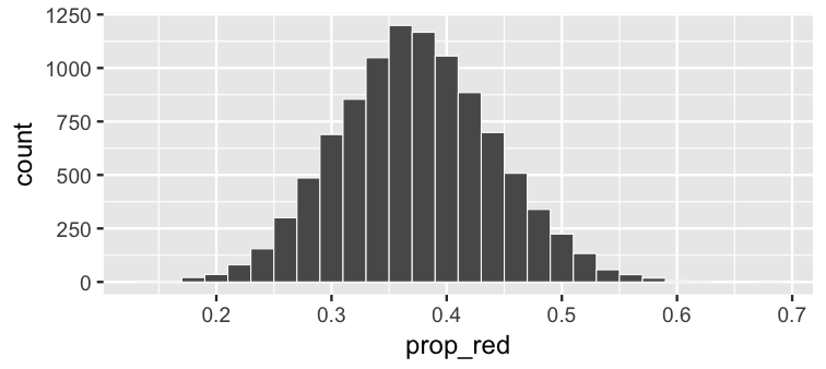
```

![](slide_deck_files/figure-html/unnamed-chunk-57-1.png)

---

# Practice

- Let's estimate the mean age of pennies
- Create a sampling distribution of 10,000 samples each of size 100 from `moderndive::pennies`

---

## Shifting focus

### What about if all we had was the one sample of balls (not the whole bowl)?

```r
jennys_sample %>% count(color)
```

```
# A tibble: 2 x 2
 color n
 <chr> <int>
1 red 19
2 white 31
```

### How could we use this sample to make a guess about the sampling variability from other samples?

---

---

# Building up to statistical inference!

```r
library(infer)
jennys_sample %>% 
  specify(formula = color ~ NULL, success = "red")
```

```
Response: color (factor)
# A tibble: 50 x 1
 color
 <fct>
 1 red 
 2 red 
 3 white
 4 white
 5 white
 6 white
 7 red 
 8 red 
 9 white
10 white
# ... with 40 more rows
```

---

# Bootstrapping?

```r
library(infer)
( bootstrap_samples <- jennys_sample %>% 
 specify(formula = color ~ NULL, success = "red") %>% 
 generate(reps = 48, type = "bootstrap") )
```

```
Response: color (factor)
# A tibble: 2,400 x 2
# Groups: replicate [48]
 replicate color
 <int> <fct>
 1 1 red 
 2 1 white
 3 1 white
 4 1 red 
 5 1 white
 6 1 white
 7 1 red 
 8 1 red 
 9 1 red 
10 1 red 
# ... with 2,390 more rows
```

---

# What does `bootstrap_samples` represent?

## Remember we assumed that all we had was the original sample of 19 red and 31 white to start.
--

## Hope `bootstrap_samples` is close to this:

---

## Bootstrap statistics

```r
jennys_sample %>% 
  specify(formula = color ~ NULL, success = "red") %>% 
  generate(reps = 48, type = "bootstrap") %>% 
  calculate(stat = "prop")
```

```
Response: color (factor)
# A tibble: 48 x 2
 replicate stat
 <int> <dbl>
 1 1 0.360
 2 2 0.320
 3 3 0.420
 4 4 0.380
 5 5 0.540
 6 6 0.260
 7 7 0.380
 8 8 0.480
 9 9 0.340
10 10 0.360
# ... with 38 more rows
```

---

## Do 10,000 reps to get a better sense for variability

### Just as we did with the sampling distribution

```r
bootstrap_stats <- jennys_sample %>% 
 specify(formula = color ~ NULL, success = "red") %>% 
 generate(reps = 10000, type = "bootstrap") %>% 
 calculate(stat = "prop")
```

---

### The bootstrap distribution

![](slide_deck_files/figure-html/unnamed-chunk-64-1.png)

### The sampling distribution

![](slide_deck_files/figure-html/unnamed-chunk-65-1.png)

---

## `infer` verbs

---

## `infer` verbs

---

.footer[Slides available at http://bit.ly/ness-infer &emsp; &emsp; &emsp; [Return to Table of Contents](#toc)]

---

# Statistical Inference

.footnote[`infer` hex sticker designs kindly created by [Thomas Mock](https://www.linkedin.com/in/jthomasmock/)]

---

.footer[Slides available at http://bit.ly/ness-infer &emsp; &emsp; &emsp; [Return to Table of Contents](#toc)]

---

# Research Question

If you see someone else yawn, are you more likely to yawn?

In an episode of the show *Mythbusters*, they tested the myth that yawning is contagious.

- Analysis done with [Alison Hill](https://alison.rbind.io)

---

## Participants and Procedure

- 50 adults who thought they were being considered for an appearance on the show.

- Each participant was interviewed individually by a show recruiter ("confederate") who either yawned or did not.

- Participants then sat by themselves in a large van and were asked to wait.

- While in the van, the Mythbusters watched to see if the unaware participants yawned.

---

## Data

- 34 saw the confederate yawn ( *seed* )
- 16 did not see the confederate yawn ( *control* )
- `1` corresponds to yawn, `0` to no yawn

```r
group <- c(rep("control", 12), rep("seed", 24), 
 rep("control", 4), rep("seed", 10))
yawn <- c(rep(0, 36), rep(1, 14))
yawn_myth <- data_frame(subj = seq(1, 50), group, yawn) %>% 
 mutate(yawn = factor(yawn))
slice(yawn_myth, c(5, 17, 37, 49))
```

```
# A tibble: 4 x 3
 subj group yawn 
 <int> <chr> <fct>
1 5 control 0 
2 17 seed 0 
3 37 control 1 
4 49 seed 1 
```

---

# Results

```r
library(janitor)
yawn_myth %>% 
  tabyl(group, yawn) %>% 
  adorn_percentages() %>% 
  adorn_pct_formatting() %>% 
  adorn_ns()
```

```
   group          0          1
 control 75.0% (12) 25.0%  (4)
    seed 70.6% (24) 29.4% (10)
```

---
class: inverse, middle, center

## Conclusion

## *Finding: CONFIRMED* 1

.footnote[
[1] http://www.discovery.com/tv-shows/mythbusters/mythbusters-database/yawning-contagious/]

---

# Really?

> "Though that's not an enormous increase, since they tested 50 people in the field, the gap was still wide enough for the MythBusters to confirm that yawning is indeed contagious." 1

.footnote[
[1] http://www.discovery.com/tv-shows/mythbusters/mythbusters-database/yawning-contagious/]

---

# State the hypotheses

Null hypothesis:

> There is no difference between the seed and control groups in the proportion of people who yawned.

Alternative hypothesis (directional):

> More people (relatively) yawned in the seed group than in the control group.

---

# Test the hypothesis

Which type of hypothesis test would you conduct here?

- Independent samples t-test
- Two proportion test
- Chi-square Goodness of Fit
- Analysis of Variance

---
class: center, middle

# Two proportion test

`$H_0: p_{seed} - p_{control} = 0$`

`$H_A: p_{seed} - p_{control} > 0$`

---

# The observed difference

```r
yawn_myth %>%
  group_by(group) %>%
  summarize(prop = mean(yawn == 1))
```

```
# A tibble: 2 x 2
 group prop
 <chr> <dbl>
1 control 0.250
2 seed 0.294
```

```r
(obs_diff <- yawn_myth %>%
 group_by(group) %>%
 summarize(prop = mean(yawn == 1)) %>%
 summarize(diff(prop)) %>%
 pull())
```

```
[1] 0.044118
```

---
class: inverse, middle, center

## Is this difference *meaningful*?

## Different question:

## Is this difference *significant*?

---

# Modeling the null hypothesis

If...

&emsp;&emsp; `$H_0: p_{seed} = p_{control}$` &emsp;&emsp;

is true, then whether or not the participant saw someone else yawn does not matter.

In other words, there is no association between exposure and yawning.

---
class: inverse, center, middle

![](http://directorsnotes.com/wp-content/uploads/2011/11/another_earth_03.jpg)
---

```
# A tibble: 12 x 3
 subj group yawn 
 <int> <chr> <fct>
 1 1 control 0 
 2 2 control 0 
 3 3 control 0 
 4 4 control 0 
 5 5 control 0 
 6 6 control 0 
 7 15 seed 0 
 8 16 seed 0 
 9 17 seed 0 
10 18 seed 0 
11 19 seed 0 
12 20 seed 0 
```

```
   group  0  1 Total
 control 12  4    16
    seed 24 10    34
   Total 36 14    50
```
]

```
# A tibble: 12 x 3
 subj group alt_yawn
 <int> <fct> <fct> 
 1 1 control 0 
 2 2 control 0 
 3 3 control 0 
 4 4 control 0 
 5 5 control 0 
 6 6 control 0 
 7 15 seed 0 
 8 16 seed 1 
 9 17 seed 1 
10 18 seed 0 
11 19 seed 0 
12 20 seed 1 
```

```
   group  0  1 Total
 control 14  2    16
    seed 22 12    34
   Total 36 14    50
```
]

---

# 1000 parallel universes

```
Response: yawn (factor)
Explanatory: group (factor)
Null Hypothesis: independence 
# A tibble: 1,000 x 2
 replicate stat
 <int> <dbl>
 1 1 0.0441
 2 2 0.0441
 3 3 -0.0478
 4 4 0.136 
 5 5 0.0441
 6 6 -0.0478
 7 7 0.136 
 8 8 -0.232 
 9 9 -0.0478
10 10 -0.0478
# ... with 990 more rows
```
]

```
# A tibble: 10 x 2
 replicate stat
 <int> <dbl>
 1 991 0.0441
 2 992 -0.0478
 3 993 0.136 
 4 994 -0.232 
 5 995 -0.140 
 6 996 -0.140 
 7 997 0.136 
 8 998 0.0441
 9 999 0.136 
10 1000 -0.324 
```
]

---
## The parallel universe distribution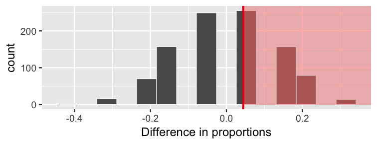

![](slide_deck_files/figure-html/unnamed-chunk-74-1.png)

The distribution of 1000 differences in proportions, if the null hypothesis were *true* and yawning was not contagious.

---
## Calculating the p-value

In how many of our "parallel universes" is the difference as big or bigger than the one we observed (0.04412)?

The shaded proportion is the p-value!

```
Response: yawn (factor)
Explanatory: group (factor)
Null Hypothesis: independence 
# A tibble: 1 x 3
 n_as_big n_total p_value
 <int> <int> <dbl>
1 505 1000 0.505
```

---
class: middle, center
layout: false

# There is Only One Test!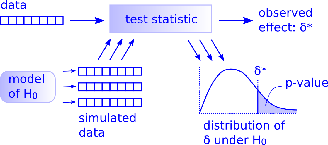

[![Only One Test](images/downey.png)](http://allendowney.blogspot.com/2016/06/there-is-still-only-one-test.html)

---

.footer[Slides available at http://bit.ly/ness-infer &emsp; &emsp; &emsp; [Return to Table of Contents](#toc)]

---

![](images/infer.073.jpeg)

---

![](images/infer.074.jpeg)

---

![](images/infer.075.jpeg)

---

![](images/infer.076.jpeg)

---

![](images/infer.077.jpeg)

---

![](images/infer.078.jpeg)

---

![](images/infer.079.jpeg)

---

![](images/infer.080.jpeg)

---

![](images/infer.081.jpeg)

---

![](images/infer.082.jpeg)

---

![](images/infer.084.jpeg)

---

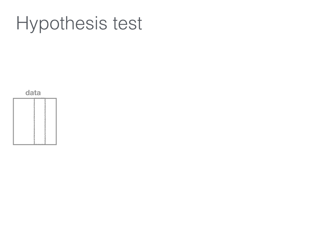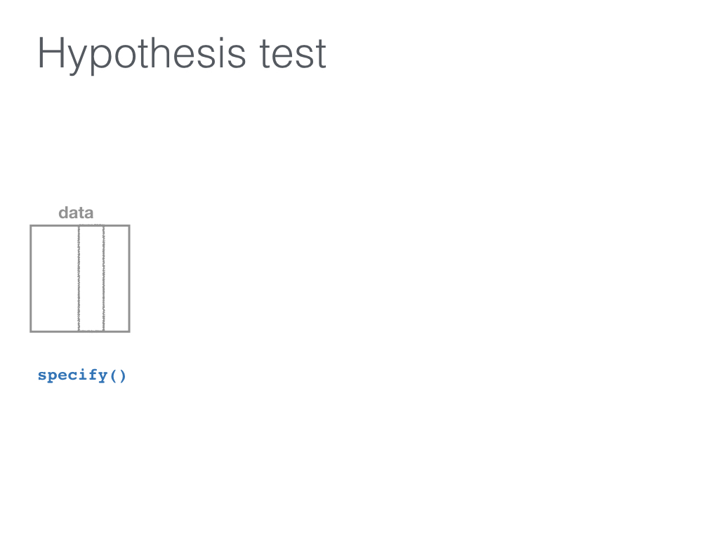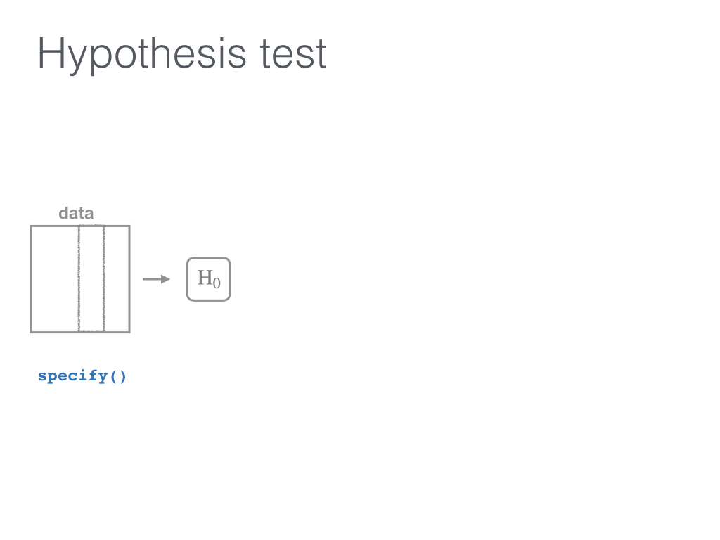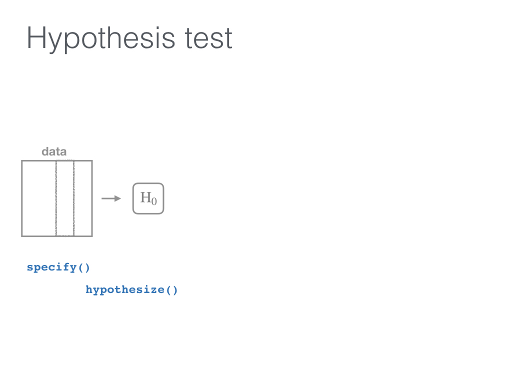.footer[Slides available at http://bit.ly/ness-infer &emsp; &emsp; &emsp; [Return to Table of Contents](#toc)]

---

# `infer`

Five functions:

- `specify()`
- `hypothesize()`
- `generate()`
- `calculate()`
- `visualize()`

---

# `infer`

- `specify` the response and explanatory variables (`y ~ x`)
- `hypothesize` what the null hypothesis is (here, `independence` of `y` and `x`)
- `generate` new samples from parallel universes under the null hypothesis model:
 - Resample from our original data without replacement, each time shuffling the `group` (`type = "permute"`)
 - Do this a ton of times (`reps = 1000`)
- `calculate` the statistic (`stat = "diff in props"`) for each of the `reps`

---

# `infer` example

```r
set.seed(8)
null_distn <- yawn_myth %>% 
 specify(formula = yawn ~ group, success = "1") %>% 
 hypothesize(null = "independence") %>% 
 generate(reps = 1000, type = "permute") %>% 
 calculate(stat = "diff in props", order = c("seed", "control"))
```

---

# Visualize the null distribution

- `visualize` the distribution of the `stat` (here, `diff in props`)

```r
null_distn %>% 
  visualize(obs_stat = obs_diff, direction = "right")
```

![](slide_deck_files/figure-html/unnamed-chunk-78-1.png)

---

# Classical inference

Rely on theory to tell us what the null distribution looks like.

```r
yawn_myth %>%
  specify(yawn ~ group, success = "1") %>%
  hypothesize(null = "independence") %>% 
  # generate() is not needed since we are not doing simulation
  calculate(stat = "z", order = c("seed", "control")) %>%
  visualize(method = "theoretical", obs_stat = obs_z,
            direction = "right")
```

---

# Classical inference

Rely on theory to tell us what the null distribution looks like.

```
Warning: Check to make sure the conditions have been met for the
theoretical method. `infer` currently does not check these for you.
```

![](slide_deck_files/figure-html/unnamed-chunk-82-1.png)

---

# Resampling vs Classical (`stat = "z"`)

```r
yawn_myth %>%
  specify(yawn ~ group, success = "1") %>%
  hypothesize(null = "independence") %>% 
  generate(reps = 1000, type = "permute") %>% 
  calculate(stat = "z", order = c("seed", "control")) %>% 
  visualize(method = "both", bins = 10, obs_stat = obs_z, 
            direction = "right")
```

```
Warning: Check to make sure the conditions have been met for the
theoretical method. `infer` currently does not check these for you.
```

![](slide_deck_files/figure-html/unnamed-chunk-83-1.png)

---

## Practice

- Read in/prep the [`mazes` data](http://bit.ly/mazes-gist)

```r
library(readr)
mazes <- read_csv("http://bit.ly/mazes-gist") %>% 
 janitor::clean_names() %>% filter(dx %in% c("ASD", "TD"))
```

- Use `infer` to compare a numerical variable between the two groups using:
 - A permutation test and
 - A classical theoretical test.
 
About the data: [Quantitative analysis of disfluency in children with autism spectrum disorder or language impairment](http://journals.plos.org/plosone/article?id=10.1371/journal.pone.0173936)

---

# More practice (time permitting)

- Find a data set / use your own and perform statistical inference on one or two of the variables there using the `infer` package

---

## More info and resources

- https://infer.netlify.com (https://infer-dev.netlify.com for development)
  - Many examples under Articles with more to come
  - To be discussed in [www.ModernDive.com](www.ModernDive.com)
      - [Sign up](http://eepurl.com/cBkItf) to the mailing list for updates
- DataCamp courses that use `infer`
  - [Inference for Numerical Data](https://www.datacamp.com/courses/inference-for-numerical-data)
  - [Inference for Regression](https://www.datacamp.com/courses/inference-for-linear-regression)
  - Two more DataCamp courses to launch soon
- [Learn the Tidyverse](https://www.tidyverse.org/learn/)

---

## Future plans

- Generalize `calculate()`'s `stat` argument
- Improve speed and memory used by shifting to list-columns
- Rewrite the inference part of the [ModernDive](http://moderndive.netlify.com/9-ci.html) book
- Lead more workshops on using the `infer` package to extend knowledge of the `tidyverse`, R, and statistics

---

## Thanks for attending! Contact me: [Email](mailto:chester@datacamp.com) or [Twitter](https://twitter.com/old_man_chester)
- Special thanks to 
 - [Albert Y. Kim](https://twitter.com/rudeboybert) 
 - [Andrew Bray](https://andrewpbray.github.io)
 - [Alison Hill](https://twitter.com/apreshill)
- Slides created via the R package [xaringan](https://github.com/yihui/xaringan) by Yihui Xie
- Slides' source code at <https://github.com/ismayc/talks/>