class: center, middle, inverse, title-slide # Statistical Inference: A Tidy Approach ## The <code><font color="black">infer</font></code> R package ### Dr. Chester Ismay <br> Senior Curriculum Lead at <a href="https://www.datacamp.com/">DataCamp</a> <br> <a href="http://github.com/ismayc"><i class="fa fa-github fa-fw"></i>  ismayc</a><br> <a href="http://twitter.com/old_man_chester"> <i class="fa fa-twitter fa-fw"></i>  <span class="citation">@old_man_chester</span></a><br> <a href="mailto:chester@datacamp.com"><i class="fa fa-paper-plane fa-fw"></i>  chester@datacamp.com</a><br> ### 2018-07-12   <img src="figure/user_au_logo_small.png" width="144" /> <br><br> Slides available at <a href="http://bit.ly/infer-useR" class="uri">http://bit.ly/infer-useR</a> <br> Package webpage at <a href="https://infer.netlify.com" class="uri">https://infer.netlify.com</a> --- class: inverse layout: true .footer[Slides available at <http://bit.ly/infer-useR> <br> Package webpage at <https://infer.netlify.com>] --- ## Understanding who you are - Who uses hypothesis testing/confidence intervals at least once a week? -- - Who uses the `tidyverse` at least once a week? -- - Who has heard of simulation-based inference methods? - Permutation testing? - Resampling methods? - Bootstrap methods? --- class: middle <small>Students at Virginia Tech studied which vehicles come to a <font color="mediumpurple">complete stop</font> at an intersection with four-way stop signs, selecting at random the cars to observe. <!--They looked at several factors to see which (if any) were associated with coming to a complete stop. (They defined a complete stop as “the speed of the vehicle will become zero at least for an [instant]”). Some of these variables included the age of the driver, how many passengers were in the vehicle, and type of vehicle.--> The <font color="lightgreen">explanatory</font> variable used here is the arrival position of vehicles approaching an intersection all traveling in the same direction. They classified this arrival pattern into three groups: whether the vehicle arrives alone (<code><small>single</small></code>), is the <code><small>lead</small></code> in a group of vehicles, or is a <code><small>follow</small></code>er in a group of vehicles. Is there an association between <font color="lightgreen">arrival pattern</font> and whether a <code><font color="purple"><small>complete</small></font></code> stop or <code><font color="purple"><small>not_complete</small></font></code> was made?</small> <!--The students studied one specific intersection in Northern Virginia at a variety of different times. Because random assignment was not used, this is an observational study. Also note that no vehicle from one group is paired with a vehicle from another group.--> <br> <tiny>- From <a href="http://math.hope.edu/isi/"> "Introduction to Statistical Investigations" </a> by Tintle et al.</tiny> --- class: middle Which type of hypothesis test should we conduct here? - A. Independent samples t-test - B. One proportion test - C. Chi-Square test of independence - D. ANOVA --- ```r library(tidyverse) # https://ismayc.github.io/talks/infer-useR/car_stop.rds download.file("http://bit.ly/car_stop_rds", destfile = "car_stop.rds") car_stop <- read_rds("car_stop.rds") car_stop %>% sample_n(10) ``` ``` # A tibble: 10 x 2 stop_type vehicle_type <chr> <chr> 1 complete single 2 complete follow 3 complete lead 4 complete single 5 not_complete follow 6 not_complete lead 7 complete single 8 complete follow 9 complete single 10 complete lead ``` --- class: middle Which type of hypothesis test should we conduct here? - A. Independent samples t-test - B. One proportion test - C. Chi-Square Test of Independence - D. ANOVA -- <br> *** ## Answer: - **C. Chi-Square Test of Independence** --- class: middle ## Let's do this in R - Using a `data` argument ```r chisq.test(data = car_stop, x = stop_type, y = vehicle_type) ``` -- ``` Error in chisq.test(data = car_stop, x = stop_type, y = vehicle_type) ``` -- - Using a formula ```r chisq.test(data = car_stop, formula = vehicle_type ~ stop_type) ``` -- ``` Error in chisq.test(data = car_stop, formula = vehicle_type ~ stop_type) ``` <br> --- ## Finally ```r chisq.test(car_stop$stop_type, car_stop$vehicle_type) ``` ``` Pearson's Chi-squared test data: car_stop$stop_type and car_stop$vehicle_type X-squared = 3.9476, df = 2, p-value = 0.1389 ``` --- layout: false ## ```r ?chisq.test() ``` [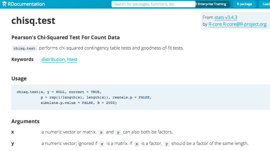](https://www.rdocumentation.org/packages/stats/versions/3.4.3/topics/chisq.test) --- class: inverse layout: true .footer[Slides available at <http://bit.ly/infer-useR> <br> Package webpage at <https://infer.netlify.com>] --- 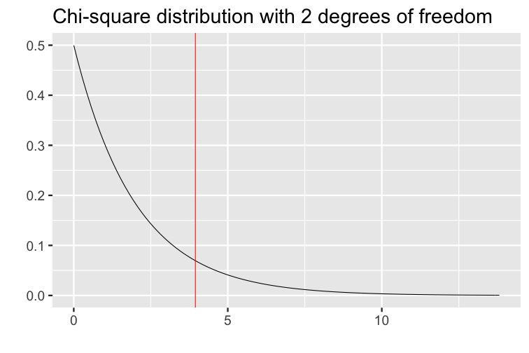<!-- --> P-value is 0.1389. --- ## `infer` Teaser - Maybe a different approach? ```r library(infer) car_stop %>% chisq_test(vehicle_type ~ stop_type) ``` ``` statistic chisq_df p_value 1 3.947648 2 0.1389246 ``` <img src="figure/v0.3.0.png" width="888" /> --- Is there an association between arrival pattern and whether or not a complete stop was made? ## The null hypothesis > No association exists between the arrival vehicle's position and whether or not it makes a complete stop. ## The alternative hypothesis > An association exists between the arrival vehicle's position and whether or not it makes a complete stop. --- layout: false ## How can computation help us to understand what is going on here? -- [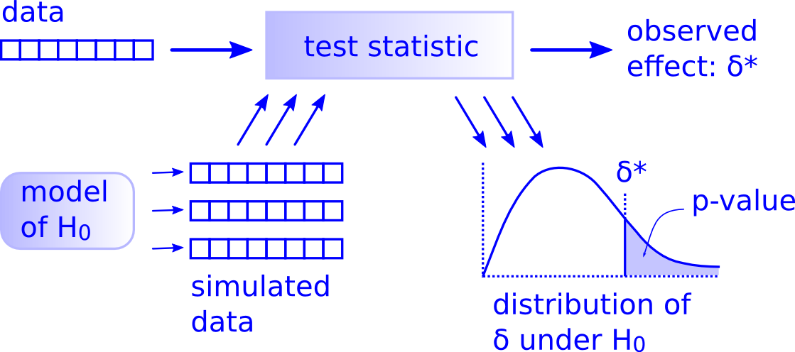](http://allendowney.blogspot.com/2016/06/there-is-still-only-one-test.html) --- class: inverse layout: true .footer[Slides available at <http://bit.ly/infer-useR> <br> Package webpage at <https://infer.netlify.com>] --- ## The tricky step -- Modeling the null hypothesis - How do we simulate data assuming the null hypothesis is true in our problem (there is no association between the variables)? -- - What might the sample data look like if the null was true? --- ### Properties of the original sample collected ```r car_stop %>% dplyr::count(stop_type, vehicle_type) ``` ``` # A tibble: 6 x 3 stop_type vehicle_type n <chr> <chr> <int> 1 complete follow 76 2 complete lead 38 3 complete single 151 4 not_complete follow 22 5 not_complete lead 5 6 not_complete single 25 ``` -- ```r ( orig_table <- car_stop %>% janitor::tabyl(stop_type, vehicle_type) ) ``` ``` stop_type follow lead single complete 76 38 151 not_complete 22 5 25 ``` --- ### Permute the sample data <br> - Shuffle `stop_type` across `vehicle_type` ``` # A tibble: 317 x 2 stop_type vehicle_type <fct> <fct> 1 complete follow 2 not_complete follow 3 complete follow 4 not_complete single 5 complete single 6 not_complete follow 7 not_complete single 8 complete follow 9 not_complete lead 10 complete lead # ... with 307 more rows ``` -- ``` stop_type follow lead single complete 79 35 151 not_complete 19 8 25 ``` --- ## Comparing the original and permuted sample ```r orig_table %>% janitor::adorn_totals(where = c("row", "col")) ``` ``` stop_type follow lead single Total complete 76 38 151 265 not_complete 22 5 25 52 Total 98 43 176 317 ``` ```r new_table %>% janitor::adorn_totals(where = c("row", "col")) ``` ``` stop_type follow lead single Total complete 79 35 151 265 not_complete 19 8 25 52 Total 98 43 176 317 ``` --- layout: false ## Where are we? [](http://allendowney.blogspot.com/2016/06/there-is-still-only-one-test.html) --- class: inverse layout: true .footer[Slides available at <http://bit.ly/infer-useR> <br> Package webpage at <https://infer.netlify.com>] --- ## Chi-square test statistic - Measure of how far what we observed in our sample is from what we would expect if the null hypothesis was true ([Wikipedia](https://en.wikipedia.org/wiki/Pearson%27s_chi-squared_test)) -- ```r car_stop %>% infer::chisq_stat(vehicle_type ~ stop_type) ``` ``` stat 1 3.947648 ``` ```r chisq.test(car_stop$stop_type, car_stop$vehicle_type)$statistic ``` ``` X-squared 3.947648 ``` --- ## For the permuted data ```r perm1 %>% infer::chisq_stat(vehicle_type ~ stop_type) ``` ``` stat 1 1.408986 ``` -- ## Another permutation ```r perm2 %>% infer::chisq_stat(vehicle_type ~ stop_type) ``` ``` stat 1 0.3604528 ``` --- ## What does the distribution of multiple repetitions of the permuted data look like? ``` # A tibble: 1,000 x 2 replicate stat <int> <dbl> 1 1 1.05 2 2 7.24 3 3 0.253 4 4 2.16 5 5 1.60 6 6 3.95 7 7 1.94 8 8 1.68 9 9 0.242 10 10 3.26 # ... with 990 more rows ``` --- layout: false <small>The distribution of multiple repetitions of the permuted data</small> 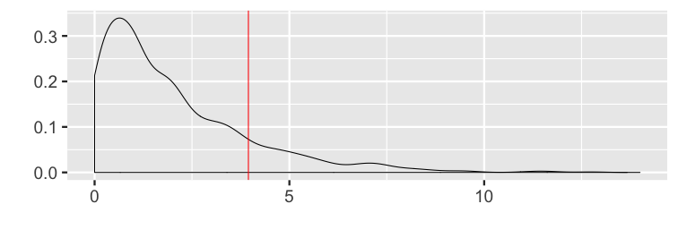<!-- --> -- <small>Recall the traditional method using the Chi-square distribution </small> <!-- --> --- class: inverse layout: true .footer[Slides available at <http://bit.ly/infer-useR> <br> Package webpage at <https://infer.netlify.com>] --- <!-- So how did I generate this code to permute? --> ## Objectives of the `infer` package - Implement common classical inferential techniques in a `tidyverse`-friendly framework that is expressive of the underlying procedure. -- - Dataframe in, dataframe out - Compose tests and intervals with pipes - Unite computational and approximation methods - Reading a chain of `infer` code should describe the inferential procedure --- layout: false class: inverse, center, middle # The `infer` verbs ---  ---  ---  --- 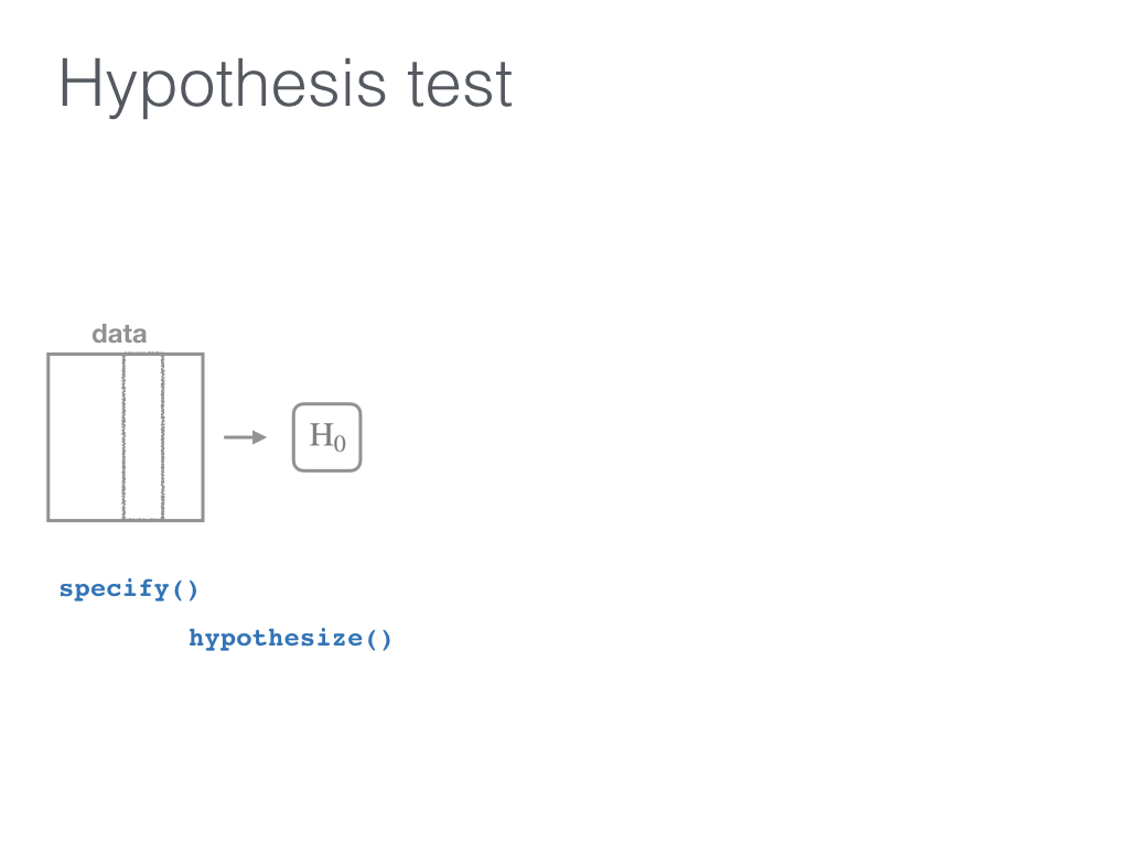 --- 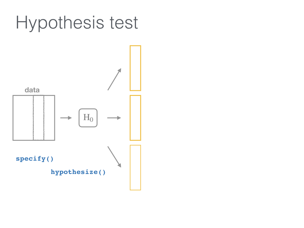 --- 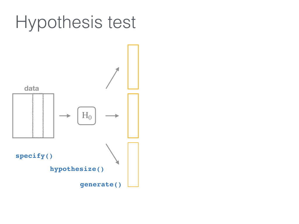 --- 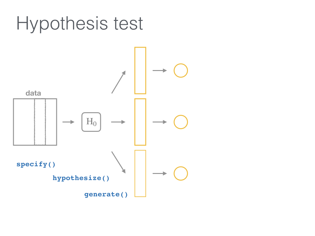 ---  ---  ---  ---  --- class: inverse layout: true .footer[Slides available at <http://bit.ly/infer-useR> <br> Package webpage at <https://infer.netlify.com>] --- ```r library(infer) car_stop %>% specify(stop_type ~ vehicle_type) %>% hypothesize(null = "independence") %>% generate(reps = 1000, type = "permute") %>% calculate(stat = "Chisq") ``` ``` # A tibble: 1,000 x 2 replicate stat <int> <dbl> 1 1 0.509 2 2 0.760 3 3 1.79 4 4 1.83 5 5 0.525 6 6 4.74 7 7 1.11 8 8 2.51 9 9 1.11 10 10 0.421 # ... with 990 more rows ``` --- ## Back to the example ```r null_distn <- car_stop %>% specify(stop_type ~ vehicle_type) %>% hypothesize(null = "independence") %>% generate(reps = 1000, type = "permute") %>% calculate(stat = "Chisq") null_distn %>% visualize() ``` <!-- --> --- ## Get the simulation-based p-value ```r Chisq_obs <- car_stop %>% specify(stop_type ~ vehicle_type) %>% calculate(stat = "Chisq") null_distn %>% get_pvalue(obs_stat = Chisq_obs, direction = "greater") ``` ``` # A tibble: 1 x 1 p_value <dbl> 1 0.13 ``` --- ## Visualize it ```r null_distn %>% visualize(obs_stat = Chisq_obs, direction = "greater") ``` <!-- --> --- ## Compare to theoretical ```r null_distn %>% visualize(method = "both", obs_stat = Chisq_obs, direction = "greater") ``` ``` Warning: Check to make sure the conditions have been met for the theoretical method. `infer` currently does not check these for you. ``` <!-- --> --- ## What's to come with `infer` - Generalized input to `calculate()` - For example, `calculate(trimmed_mean)` - [More to-dos](https://infer-dev.netlify.com/to-do) - Feature requests and bug reports at https://github.com/andrewpbray/infer/issues --- class: inverse layout: false ## More info and practice - [infer.netlify.com](https://infer.netlify.com) (or [infer-dev.netlify.com](https://infer-dev.netlify.com)) - Many examples under Articles with more to come - To be fully implemented in [ModernDive.com](www.ModernDive.com) - [Sign up](http://eepurl.com/cBkItf) for the ModernDive mailing list - DataCamp courses with `infer` + one more coming - [Inference for Numerical Data](https://www.datacamp.com/courses/inference-for-numerical-data) - [Inference for Categorical Data](https://www.datacamp.com/courses/inference-for-categorical-data) - [Inference for Regression](https://www.datacamp.com/courses/inference-for-linear-regression) - Keep an eye on the [`tidymodels` meta-package](https://github.com/tidymodels/tidymodels) --- layout: false class: inverse, middle <center> <a href="https://www.tidyverse.org/learn"> <img src="figure/tidyverse.png" style="width: 200px;"/> </a>&emsp;&emsp;<a href="https://moderndive.netlify.com"> <img src="figure/dark_vert.png" style="width: 221px;"/></a>&emsp;&emsp;<a href="https://infer.netlify.com"> <img src="figure/infer_gnome.png" style="width: 230px;"/></a></center> ## Thanks for attending! Contact me: [Email](mailto:chester@datacamp.com) or [Twitter](https://twitter.com/old_man_chester) - Thanks to [Albert Y. Kim](https://twitter.com/rudeboybert), [Andrew Bray](https://andrewpbray.github.io), and [Alison Hill](https://twitter.com/apreshill) - Slides created via the R package [xaringan](https://github.com/yihui/xaringan) by Yihui Xie - Slides' source code at <https://github.com/ismayc/talks/>