Tidyverse Tools in R for Data Science and Statistical Inference

# Tidyverse Tools in R for <br> Data Science and Statistical Inference

## Dr. Jessica Minnier and Dr. Chester Ismay

### Slides available at <http://bit.ly/csp-tidy-slides>

### PDF slides at <http://bit.ly/csp-tidy-pdf>

???

Welcome to our course! You can find the link to the HTML version of our slides
as well as the PDF version here. We'll give you a few minutes to get these
loaded and then start with introductions of your presenters.

---

.pull-left[
  <img class="circle" src="https://github.com/jminnier.png" width="200px"/>
  
  <small>Associate Professor of Biostatistics</small>
  
  <img src="images/ohsu_logo.jpg" width="80px"/>

<br>

[<svg style="height:0.8em;top:.04em;position:relative;" viewBox="0 0 512 512"><path d="M459.37 151.716c.325 4.548.325 9.097.325 13.645 0 138.72-105.583 298.558-298.558 298.558-59.452 0-114.68-17.219-161.137-47.106 8.447.974 16.568 1.299 25.34 1.299 49.055 0 94.213-16.568 130.274-44.832-46.132-.975-84.792-31.188-98.112-72.772 6.498.974 12.995 1.624 19.818 1.624 9.421 0 18.843-1.3 27.614-3.573-48.081-9.747-84.143-51.98-84.143-102.985v-1.299c13.969 7.797 30.214 12.67 47.431 13.319-28.264-18.843-46.781-51.005-46.781-87.391 0-19.492 5.197-37.36 14.294-52.954 51.655 63.675 129.3 105.258 216.365 109.807-1.624-7.797-2.599-15.918-2.599-24.04 0-57.828 46.782-104.934 104.934-104.934 30.213 0 57.502 12.67 76.67 33.137 23.715-4.548 46.456-13.32 66.599-25.34-7.798 24.366-24.366 44.833-46.132 57.827 21.117-2.273 41.584-8.122 60.426-16.243-14.292 20.791-32.161 39.308-52.628 54.253z"/></svg> @datapointier](http://twitter.com/datapointier)  
  [<svg style="height:0.8em;top:.04em;position:relative;" viewBox="0 0 496 512"><path d="M165.9 397.4c0 2-2.3 3.6-5.2 3.6-3.3.3-5.6-1.3-5.6-3.6 0-2 2.3-3.6 5.2-3.6 3-.3 5.6 1.3 5.6 3.6zm-31.1-4.5c-.7 2 1.3 4.3 4.3 4.9 2.6 1 5.6 0 6.2-2s-1.3-4.3-4.3-5.2c-2.6-.7-5.5.3-6.2 2.3zm44.2-1.7c-2.9.7-4.9 2.6-4.6 4.9.3 2 2.9 3.3 5.9 2.6 2.9-.7 4.9-2.6 4.6-4.6-.3-1.9-3-3.2-5.9-2.9zM244.8 8C106.1 8 0 113.3 0 252c0 110.9 69.8 205.8 169.5 239.2 12.8 2.3 17.3-5.6 17.3-12.1 0-6.2-.3-40.4-.3-61.4 0 0-70 15-84.7-29.8 0 0-11.4-29.1-27.8-36.6 0 0-22.9-15.7 1.6-15.4 0 0 24.9 2 38.6 25.8 21.9 38.6 58.6 27.5 72.9 20.9 2.3-16 8.8-27.1 16-33.7-55.9-6.2-112.3-14.3-112.3-110.5 0-27.5 7.6-41.3 23.6-58.9-2.6-6.5-11.1-33.3 2.6-67.9 20.9-6.5 69 27 69 27 20-5.6 41.5-8.5 62.8-8.5s42.8 2.9 62.8 8.5c0 0 48.1-33.6 69-27 13.7 34.7 5.2 61.4 2.6 67.9 16 17.7 25.8 31.5 25.8 58.9 0 96.5-58.9 104.2-114.8 110.5 9.2 7.9 17 22.9 17 46.4 0 33.7-.3 75.4-.3 83.6 0 6.5 4.6 14.4 17.3 12.1C428.2 457.8 496 362.9 496 252 496 113.3 383.5 8 244.8 8zM97.2 352.9c-1.3 1-1 3.3.7 5.2 1.6 1.6 3.9 2.3 5.2 1 1.3-1 1-3.3-.7-5.2-1.6-1.6-3.9-2.3-5.2-1zm-10.8-8.1c-.7 1.3.3 2.9 2.3 3.9 1.6 1 3.6.7 4.3-.7.7-1.3-.3-2.9-2.3-3.9-2-.6-3.6-.3-4.3.7zm32.4 35.6c-1.6 1.3-1 4.3 1.3 6.2 2.3 2.3 5.2 2.6 6.5 1 1.3-1.3.7-4.3-1.3-6.2-2.2-2.3-5.2-2.6-6.5-1zm-11.4-14.7c-1.6 1-1.6 3.6 0 5.9 1.6 2.3 4.3 3.3 5.6 2.3 1.6-1.3 1.6-3.9 0-6.2-1.4-2.3-4-3.3-5.6-2z"/></svg> @jminnier](http://github.com/jminnier)  
  [<svg style="height:0.8em;top:.04em;position:relative;" viewBox="0 0 512 512"><path d="M326.612 185.391c59.747 59.809 58.927 155.698.36 214.59-.11.12-.24.25-.36.37l-67.2 67.2c-59.27 59.27-155.699 59.262-214.96 0-59.27-59.26-59.27-155.7 0-214.96l37.106-37.106c9.84-9.84 26.786-3.3 27.294 10.606.648 17.722 3.826 35.527 9.69 52.721 1.986 5.822.567 12.262-3.783 16.612l-13.087 13.087c-28.026 28.026-28.905 73.66-1.155 101.96 28.024 28.579 74.086 28.749 102.325.51l67.2-67.19c28.191-28.191 28.073-73.757 0-101.83-3.701-3.694-7.429-6.564-10.341-8.569a16.037 16.037 0 0 1-6.947-12.606c-.396-10.567 3.348-21.456 11.698-29.806l21.054-21.055c5.521-5.521 14.182-6.199 20.584-1.731a152.482 152.482 0 0 1 20.522 17.197zM467.547 44.449c-59.261-59.262-155.69-59.27-214.96 0l-67.2 67.2c-.12.12-.25.25-.36.37-58.566 58.892-59.387 154.781.36 214.59a152.454 152.454 0 0 0 20.521 17.196c6.402 4.468 15.064 3.789 20.584-1.731l21.054-21.055c8.35-8.35 12.094-19.239 11.698-29.806a16.037 16.037 0 0 0-6.947-12.606c-2.912-2.005-6.64-4.875-10.341-8.569-28.073-28.073-28.191-73.639 0-101.83l67.2-67.19c28.239-28.239 74.3-28.069 102.325.51 27.75 28.3 26.872 73.934-1.155 101.96l-13.087 13.087c-4.35 4.35-5.769 10.79-3.783 16.612 5.864 17.194 9.042 34.999 9.69 52.721.509 13.906 17.454 20.446 27.294 10.606l37.106-37.106c59.271-59.259 59.271-155.699.001-214.959z"/></svg> jessicaminnier.com](https:/jessicaminnier.com)  

]

.pull-right[
  <img class="circle" src="https://github.com/ismayc.png" width="200px"/>
  
  <small>Data Science Evangelist</small>
  
  <br>
  
  <img src="images/datarobot_logo.png" width="150px"/>
  
  <br><br>
  
  [<svg style="height:0.8em;top:.04em;position:relative;" viewBox="0 0 512 512"><path d="M459.37 151.716c.325 4.548.325 9.097.325 13.645 0 138.72-105.583 298.558-298.558 298.558-59.452 0-114.68-17.219-161.137-47.106 8.447.974 16.568 1.299 25.34 1.299 49.055 0 94.213-16.568 130.274-44.832-46.132-.975-84.792-31.188-98.112-72.772 6.498.974 12.995 1.624 19.818 1.624 9.421 0 18.843-1.3 27.614-3.573-48.081-9.747-84.143-51.98-84.143-102.985v-1.299c13.969 7.797 30.214 12.67 47.431 13.319-28.264-18.843-46.781-51.005-46.781-87.391 0-19.492 5.197-37.36 14.294-52.954 51.655 63.675 129.3 105.258 216.365 109.807-1.624-7.797-2.599-15.918-2.599-24.04 0-57.828 46.782-104.934 104.934-104.934 30.213 0 57.502 12.67 76.67 33.137 23.715-4.548 46.456-13.32 66.599-25.34-7.798 24.366-24.366 44.833-46.132 57.827 21.117-2.273 41.584-8.122 60.426-16.243-14.292 20.791-32.161 39.308-52.628 54.253z"/></svg> @old_man_chester](http://twitter.com/old_man_chester)  
  [<svg style="height:0.8em;top:.04em;position:relative;" viewBox="0 0 496 512"><path d="M165.9 397.4c0 2-2.3 3.6-5.2 3.6-3.3.3-5.6-1.3-5.6-3.6 0-2 2.3-3.6 5.2-3.6 3-.3 5.6 1.3 5.6 3.6zm-31.1-4.5c-.7 2 1.3 4.3 4.3 4.9 2.6 1 5.6 0 6.2-2s-1.3-4.3-4.3-5.2c-2.6-.7-5.5.3-6.2 2.3zm44.2-1.7c-2.9.7-4.9 2.6-4.6 4.9.3 2 2.9 3.3 5.9 2.6 2.9-.7 4.9-2.6 4.6-4.6-.3-1.9-3-3.2-5.9-2.9zM244.8 8C106.1 8 0 113.3 0 252c0 110.9 69.8 205.8 169.5 239.2 12.8 2.3 17.3-5.6 17.3-12.1 0-6.2-.3-40.4-.3-61.4 0 0-70 15-84.7-29.8 0 0-11.4-29.1-27.8-36.6 0 0-22.9-15.7 1.6-15.4 0 0 24.9 2 38.6 25.8 21.9 38.6 58.6 27.5 72.9 20.9 2.3-16 8.8-27.1 16-33.7-55.9-6.2-112.3-14.3-112.3-110.5 0-27.5 7.6-41.3 23.6-58.9-2.6-6.5-11.1-33.3 2.6-67.9 20.9-6.5 69 27 69 27 20-5.6 41.5-8.5 62.8-8.5s42.8 2.9 62.8 8.5c0 0 48.1-33.6 69-27 13.7 34.7 5.2 61.4 2.6 67.9 16 17.7 25.8 31.5 25.8 58.9 0 96.5-58.9 104.2-114.8 110.5 9.2 7.9 17 22.9 17 46.4 0 33.7-.3 75.4-.3 83.6 0 6.5 4.6 14.4 17.3 12.1C428.2 457.8 496 362.9 496 252 496 113.3 383.5 8 244.8 8zM97.2 352.9c-1.3 1-1 3.3.7 5.2 1.6 1.6 3.9 2.3 5.2 1 1.3-1 1-3.3-.7-5.2-1.6-1.6-3.9-2.3-5.2-1zm-10.8-8.1c-.7 1.3.3 2.9 2.3 3.9 1.6 1 3.6.7 4.3-.7.7-1.3-.3-2.9-2.3-3.9-2-.6-3.6-.3-4.3.7zm32.4 35.6c-1.6 1.3-1 4.3 1.3 6.2 2.3 2.3 5.2 2.6 6.5 1 1.3-1.3.7-4.3-1.3-6.2-2.2-2.3-5.2-2.6-6.5-1zm-11.4-14.7c-1.6 1-1.6 3.6 0 5.9 1.6 2.3 4.3 3.3 5.6 2.3 1.6-1.3 1.6-3.9 0-6.2-1.4-2.3-4-3.3-5.6-2z"/></svg> @ismayc](http://github.com/ismayc)  
  [<svg style="height:0.8em;top:.04em;position:relative;" viewBox="0 0 512 512"><path d="M326.612 185.391c59.747 59.809 58.927 155.698.36 214.59-.11.12-.24.25-.36.37l-67.2 67.2c-59.27 59.27-155.699 59.262-214.96 0-59.27-59.26-59.27-155.7 0-214.96l37.106-37.106c9.84-9.84 26.786-3.3 27.294 10.606.648 17.722 3.826 35.527 9.69 52.721 1.986 5.822.567 12.262-3.783 16.612l-13.087 13.087c-28.026 28.026-28.905 73.66-1.155 101.96 28.024 28.579 74.086 28.749 102.325.51l67.2-67.19c28.191-28.191 28.073-73.757 0-101.83-3.701-3.694-7.429-6.564-10.341-8.569a16.037 16.037 0 0 1-6.947-12.606c-.396-10.567 3.348-21.456 11.698-29.806l21.054-21.055c5.521-5.521 14.182-6.199 20.584-1.731a152.482 152.482 0 0 1 20.522 17.197zM467.547 44.449c-59.261-59.262-155.69-59.27-214.96 0l-67.2 67.2c-.12.12-.25.25-.36.37-58.566 58.892-59.387 154.781.36 214.59a152.454 152.454 0 0 0 20.521 17.196c6.402 4.468 15.064 3.789 20.584-1.731l21.054-21.055c8.35-8.35 12.094-19.239 11.698-29.806a16.037 16.037 0 0 0-6.947-12.606c-2.912-2.005-6.64-4.875-10.341-8.569-28.073-28.073-28.191-73.639 0-101.83l67.2-67.19c28.239-28.239 74.3-28.069 102.325.51 27.75 28.3 26.872 73.934-1.155 101.96l-13.087 13.087c-4.35 4.35-5.769 10.79-3.783 16.612 5.864 17.194 9.042 34.999 9.69 52.721.509 13.906 17.454 20.446 27.294 10.606l37.106-37.106c59.271-59.259 59.271-155.699.001-214.959z"/></svg> chester.rbind.io](https://chester.rbind.io)  

]

???

Hello. My name is Chester and I lead data science and machine learning courses
for DataRobot. I'm based in Portland, Oregon. I'm next going to give you an
overview of the content of this course and review R prerequisites to follow
along with us before I turn it back over to Jessica
to lead you through the first part of the course.

---

Part 1
- [Introduction and Setup](#getting-started)
- [Data Wrangling](#wrangling)
- [Data Visualization Basics](#viz)

Part 2
- [Sampling](#sampling)
- [Inference](#inference)

???
The first part of the course is focused on exploratory data analysis in
the tidyverse and the second part is about statistical inference using
data science principles you'll learn about in the first part.
---

<div class="my-footer"><span>Slides at https://bit.ly/csp-tidy-slides &emsp; &emsp; &emsp; &emsp; &emsp; &emsp; &emsp; &emsp; &emsp; Return to <u><a style="color:White;" href="slide_deck.html#toc">Table of Contents</a></u></span></div>

---

name:getting-started

## Prior Installation

Make sure you have the current R, RStudio, & R packages
- [Novice's Guide](https://moderndive.com/1-getting-started.html) on ModernDive.com

???
We recommend that you have the following versions of R, RStudio, and some R
packages downloaded. If you are having issues getting these things going right
now, we recommend you just follow along with the slides and work to get the
installations working during exercises and our break about halfway through.

***

- [R (version 4.0.2 or greater)](https://cloud.r-project.org/)
- [RStudio (version 1.4 or greater)](https://www.rstudio.com/products/rstudio/download3/)

***

<!--
These slides were built using

```r
R.version.string
```

```
[1] "R version 4.0.3 (2020-10-10)"
```

```r
rstudioapi::versionInfo()$version
```

```
[1] '1.4.461'
```
-->

<br>

- Run this in the RStudio Console

```r
pkgs <- c(
  "tidyverse", "moderndive", "dslabs", 
  "infer", "janitor", "usethis"
  )
install.packages(pkgs)
```

???
If you already downloaded the course materials and already ran the prereqs.R,
you can skip running this code again. After you've run these commands to get the packages installed, please follow
the steps on the next slide. I'll leave this up for a little bit to make sure
those following along can copy the code into RStudio and run it.

---

# Getting started

**1.** Open HTML slides: <https://bit.ly/csp-tidy-slides>

**2.** Open RStudio

**3.** Download course materials to your preferred location by copying this
and running it in the RStudio Console:

```r
usethis::use_course("https://csp2021.netlify.app/materials.zip")
```

**4.** Edit Google Doc to ask and answer questions:
[https://bit.ly/csp-tidy-doc](https://docs.google.com/document/d/1Qsf1-GNMkjkP7lQAdiuhuu-gEP2reS2vkxRwfdXdYUI/edit)

???
- Just a reminder here on the HTML slides link if you missed it at the beginning.
It will also be available at the bottom of the slides as you can see here
throughout the presentation.

- Please follow steps 2 and 3 next including copying the code in step 3 and
running in RStudio. This will start up a new RStudio project and make sure
you have the code available that we will go over.

- Lastly please open up the Google Doc linked here. You can add your questions
and any issues you are having here. We'll be keeping an eye on it. Help out
your fellow participants as well if you are able to answer questions before
Jessica or I can.

- I'm going to turn it over to Jessica now to get us going
on the content.
---

# R Data Types

???

Great, so we are assuming you have some experience with R, and so hopefully you are familiar with the various data types in R.

---

## Data types review

Vector/variable
  - Type of vector (`int`, `num` or `dbl`, `chr`, `lgl`, `date`)

???

- But just as a refresher, the main components we work with are called vectors, which store a certain variable type, either from our data, or for other computational uses. So we have integer and numeric, also called double, which store numbers, as well as character for letters or words etc, as well as logical for true/false or boolean data, and date. You will probably encounter numeric and character most often, and date is useful for timestamp tor dates.
- Usually our data is basically a set of vectors or variables, and often of different types. In R, we store those in a data frame, which is essentially a rectangular data table or matrix, with information about different kinds of variables. We think of data frames as having observations usually by row, and so each vector in a data frame must have the same number of rows.
--

Data frame
  - Vectors of (potentially) different types
  - Each vector has the same number of rows

---

## Data types review

```r
library(tibble) # tibble is the tidyverse data.frame
library(lubridate)
ex1 <- tibble(
  vec1 = c(1980, 1990, 2000, 2010),
  vec2 = c(1L, 2L, 3L, 4L),
  vec3 = c("low", "low", "high", "high"),
  vec4 = c(TRUE, FALSE, FALSE, FALSE),
  vec5 = ymd(c("2017-05-23", "1776/07/04", 
               "1983-05/31", "1908/04-01"))
)
ex1
```

???

- So if you have worked in R, you should have worked with data frames, and when you made a new data frame by hand you likely used the function data.frame. In the tidyverse, we use a different flavor of data frame called a tibble. Basically, it is a  data frame with some extra information and features. We can use the function tibble to create it. 
- Then, when we print out the new tibble, or fancy data frame, we can see the output tells us it is a tibble, it tells us the number of rows and columns, and we also see the variable or vector types at the top of the data frame. We don’t get this information automatically from a regular data frame. For all intents and purposes this acts like a data frame when doing analyses or data wrangling. The most noticable differences are usually in just how it is printed. Something you can’t see here is that if we had three thousand rows in this tibble, it would only print the top 10 or so. If you’ve ever accidentally printed a giant data frame in R, you know that the default way is to print all the rows, which is a bit annoying. So tibbles fix annoying things like that.
- We show you this, because when using the tidyverse functions, the output is going to be a tibble. Also, when you use tidyverse functions to read in data, such as read underscore excel, or read underscore table, the resulting data frame is actually a tibble. So just something to be aware of.
--

```
# A tibble: 4 x 5
   vec1  vec2 vec3  vec4  vec5      
  <dbl> <int> <chr> <lgl> <date>    
1  1980     1 low   TRUE  2017-05-23
2  1990     2 low   FALSE 1776-07-04
3  2000     3 high  FALSE 1983-05-31
4  2010     4 high  FALSE 1908-04-01
```
  
---

## Learning objectives

### Part 1

- Distinguish between different {tidyverse} packages
- Assess different {dplyr} functions for wrangling data
- Discuss the power of "tidy data"
- Develop an intuition behind {ggplot2} plotting syntax

???

Ok, so just a note about going forward and our goals for this super short introduction to tidyverse in the first hour. We want to talk about the differences between different tidyverse packages and look at different functions in the dplyr package for wrangling data. We will talk a bit about tidy data, and an extremely short intro to ggplot, really just a taste to get you interested in finding out more.

---

### Shameless plug

???

Ok this is Chester’s shameless plug in that most of what we are talking about today is in this awesome book that Chester and his colleagues wrote, called Modern Dive. It’s available freely online at this websote, and was also recently published in book form as well. So if you want to learn more through reading and exercises, I definitely recommend it, and I can say that because I had nothing to do with it.

---

# Getting started with {dplyr}

<br>

[Alison Horst](https://github.com/allisonhorst/stats-illustrations) 
]

[dplyr package](https://dplyr.tidyverse.org)
]

???
Now, the first main tidyverse package we will talk about is dplyr, which is mainly for what we call data wrangling. 
---

class: center, middle  
  
## Welcome to the [tidyverse](https://blog.rstudio.org/2016/09/15/tidyverse-1-0-0/)!
  
The {tidyverse} is a collection of R packages that share common philosophies 
and are designed to work together. <br><br> 
  
<center>
<a href="https://tidyverse.tidyverse.org">
<img src="images/tidyverse_hex.png" style = "width: 200px;"/>
</a>
</center>

???

We keep mentioning the tidyverse, but we haven’t actually defined that. So in general, the tidyverse refers to a collection of R packages that share common philosophies, mainly related to what we call tidy data and how functions are written, and they are designed to work together. The tidyverse became its own package somewhat recently, so that when you install the tidyverse package, it installs a small collection of packages. But there are many other packages that fit into the tidyverse universe, they just aren’t automatically installed with the tidyverse package. 
---

## First motivating example for today

- Inspired by the late, great [Hans Rosling](https://www.youtube.com/watch?v=jbkSRLYSojo)

???

- So before we talk about code, we want to motivate you with what we are trying to achieve with our data wrangling and visualization tools in the tidyverse. We won’t be able to get into detail on how to create a plot like this in an hour or two, but just know that once you have the foundation that we talk about today, it’s not too much more work to get to a pretty amazing visual like this. Here we have an animated visualization of income per capita vs life expectancy over the years from the gapminder data set which we will use today. This plot specifically is inspired by a talk the swedish physician Hans Rosling gave, and we recommend you spend some time watching his talks because he was a really great orator and conveyer of information with data and statistics.
- So the ultimate goal is really to convey information with our data, in an intuitive way.

---

## The `gapminder` data set in {dslabs}

```r
library(dslabs)
library(dplyr)
gapminder <- tibble(gapminder)
glimpse(gapminder)
```

```
Rows: 10,545
Columns: 9
$ country          <fct> Albania, Algeria, Angola, Antigua and…
$ year             <int> 1960, 1960, 1960, 1960, 1960, 1960, 1…
$ infant_mortality <dbl> 115.40, 148.20, 208.00, NA, 59.87, NA…
$ life_expectancy  <dbl> 62.87, 47.50, 35.98, 62.97, 65.39, 66…
$ fertility        <dbl> 6.19, 7.65, 7.32, 4.43, 3.11, 4.55, 4…
$ population       <dbl> 1636054, 11124892, 5270844, 54681, 20…
$ gdp              <dbl> NA, 1.3828e+10, NA, NA, 1.0832e+11, N…
$ continent        <fct> Europe, Africa, Africa, Americas, Ame…
$ region           <fct> Southern Europe, Northern Africa, Mid…
```

- Also check out [the {gapminder} package](https://github.com/jennybc/gapminder)

???

- So that visualization was from the gapminder data, which is a free public data set from the world bank. It’s very large and all of it is available on the gapminder website, but some of it has been packaged up into an R data set. Here we are using a relatively small subset of the data found in dslabs package, but more data can be found in the gapminder package. In this data, we have about 10 thousand rows where each row or observation is for a country for one year, and we have information about those countries’ population size, infant mortality and life expectancy, and fertility rates, as well as gdp and where in the world that country is located.
- We are going to use this data for some exercises, so if you all could open an R script or R markdown or whatever you use in R and copy this code and run it right now, that will help for later.
---

## What is data wrangling?

.pull-left[
- "data janitor work"
- importing data
- cleaning data
- changing shape of data
]
.pull-right[
- fixing errors and poorly formatted data elements
- transforming columns and rows
- filtering, subsetting
]

<br>

???

- In this first hour we are mostly talking about data wrangling. By data wrangling, we mean anything we do to manipulate data to get it ready for analyses or visualization, whether that’s what we think of as data cleaning, or changing the shape or filtering of the data, or transforming or fixing up the data in some way. 
- In this diagram we can see that data wrangling includes the import, tidying, and transformation of the data before the downstream visualize and model steps.  But we also might wrangle data that has been output from model steps, so it’s actually an integral step that happens throughout the entire data analysis process, and not just at the beginning.

---

## Base R versus the {tidyverse}

- The mean life expectancy across all years for Asia

???

- Now, how does working in the tidyverse differ from working in base R.
- CLICK: First let’s look at this simple example where we want to calculate the mean life expectancy across all years for the continent of Asia. In regular base R, we need to subset the data to get only rows where continent is equal to Asia, and the common way to do this is by putting a true false statement inside the bracket. Of course there are lots of ways to do this, maybe using the subset function, but I think this is probably the most common way we are taught. Since we are subsetting rows this goes in the first slot of the bracket, and we put a comma after and then a blank to get all the columns. Then, we need to calculate the mean of the column life expectancy. This works well.
- However, we have to admit this is hard to read, and confusing for beginners because the bracket, comma thing is not so intuitive.
- CLICK: In the tidy verse, using the dplyr package, we use what is called a pipe function, which is thisfunny symbol with percent greater than percent, to essentially chain together functions. We will explain this code in more detail, but this is what we’d do in the tidyverse, where we’d run this code to perform functions in order: first filtering rows where continent equals Asia, then summarizing to get the mean life expectancy. We end up with the same answer, though note the output is a tibble.
--

```r
# Base R
asia <- gapminder[gapminder$continent == "Asia", ]
mean(asia$life_expectancy)
```

```
[1] 65.901
```
--

```r
library(dplyr)
gapminder %>%
  filter(continent == "Asia") %>%
  summarize(mean_exp = mean(life_expectancy))
```

```
# A tibble: 1 x 1
  mean_exp
     <dbl>
1     65.9
```

---

## The pipe `%>%`

???

- let’s go through that code more in detail. first, what is this pipe? Like i mentioned, this is a way to chain together commands. In R, when running multiple functions, we often end up with a web of nested parantheses, or many rows where we save the output of one function and run a new function on it, and again and again. This is a way to do that just with one symbol, the pipe. When looking at code we read it as “and then”. 
- CLICK So for this example, we use the gapminder data, and then we filter by continent, and then we summarize with mean life expectancy. So here we are able to separate out our steps using the pipe, in the order that we perform these wrangling steps.
- If you’re in rstudio there’s also a keyboard shortcut, which is cmd-shift-m on a mac, or ctrl-shift-m on windows.

- A way to chain together commands
- Can be read as "and then" when reading over code
--

```r
library(dplyr)
gapminder %>%
  filter(continent == "Asia") %>%
  summarize(mean_exp = mean(life_expectancy))
```

---

## `filter()` rows that satisfy specified conditions

???

Digging deeper into that code, the first function we use (besides the pipe, which is technically a function in the same way the plus sign or bracket are functions), but the first data wrangling function we use is the filter function, which filters rows that satisfy specified conditions. We can have multiple conditions, strung together with logical operators like the & symbol, or or symbol, or other ways you might create a true false statement. This is similar to what you might put in the brackets using the base R way we showed earlier. We will talk a bit about these logical operators in the next slides.

---

## `dplyr::filter()`

- Arguments are "filters" that you'd like to apply.

???

- Here is an example where we want to filter on year. The arguments are going to be the filters that we want to apply.
- CLICK  Note that we have to use the double equal sign to tell R we want a true/false statement. We can also see the output of the filter statement is again a tibble, this time with fewer rows because we’ve only taken the subset with year equal to 2014. Using the pipe however lets us easily keep going with our functions and we don’t really need to save this subset data to do our next step.

```r
gap_2014 <- gapminder %>% filter(year == 2014)
gap_2014
```

```
# A tibble: 185 x 9
  country              year infant_mortality life_expectancy
  <fct>               <int>            <dbl>           <dbl>
1 Albania              2014             12.9            77.9
2 Algeria              2014             22              76.3
3 Angola               2014             98.8            59.2
4 Antigua and Barbuda  2014              6.1            76.3
5 Argentina            2014             11.5            76.3
# … with 180 more rows, and 5 more variables: fertility <dbl>,
#   population <dbl>, gdp <dbl>, continent <fct>, region <fct>
```

- Use `==` to compare a variable to a value

---

## Logical operators

- Use `|` to check for any in multiple filters being true:

???

- We had an example using the & logical operator to string two logical statements together, but there is also the or operator which is this vertical line. 
- CLICK: So we would check here whether life expectancy is less than 50 OR fertility is greater than 4, one or the other or both.
- CLICK: And again we can see the tibble output, where some rows for instance the first one, does not meet the life expectancy criteria but it does meet the fertility >4 criteria.

```r
gapminder %>%
  filter(life_expectancy < 50 | fertility > 4) %>%
  slice_sample(n = 8)
```
--

```
# A tibble: 8 x 9
  country        year infant_mortality life_expectancy fertility
  <fct>         <int>            <dbl>           <dbl>     <dbl>
1 Nepal          1996             73.1            62.5      4.6 
2 Uganda         2010             49.5            57.8      6.16
3 Nicaragua      1988             54.5            71.4      4.99
4 Guinea-Bissau  1962             NA              43.6      5.67
5 Oman           1985             50.4            68.4      8.22
6 Comoros        1970            152.             48.6      7.06
7 Tajikistan     1980            100.             64.3      5.66
8 Gabon          1990             60.5            59.5      5.42
# … with 4 more variables: population <dbl>, gdp <dbl>,
#   continent <fct>, region <fct>
```

---

## Logical operators

- Use `,` to check for all of multiple filters being true:

???

- Instead of using &, we can also use commas in the filter function to check that all filters are true. 
- CLICK So here the comma is like an and, so that we need life expectancy to be less than 50 AND fertility to be greater than 4.

```r
gapminder %>%
  filter(life_expectancy < 50, fertility > 4)
```

```
# A tibble: 8 x 9
  country       year infant_mortality life_expectancy fertility
  <fct>        <int>            <dbl>           <dbl>     <dbl>
1 Algeria       1960             148.            47.5      7.65
2 Angola        1960             208             36.0      7.32
3 Bangladesh    1960             176.            46.2      6.73
4 Benin         1960             187.            38.3      6.28
5 Bhutan        1960             175             35.9      6.67
6 Bolivia       1960             173.            43.8      6.7 
7 Burkina Faso  1960             161.            35.2      6.29
8 Burundi       1960             145.            40.6      6.95
# … with 4 more variables: population <dbl>, gdp <dbl>,
#   continent <fct>, region <fct>
```

---

## Logical operators

- Use `%in%` to check for any being true <br> (shortcut to using `|` repeatedly with `==`)

???

- Another useful operator is the in operator, which checks whether one thing is in a vector of things. 
- CLICK: So here we want country to be in one of these countries, and year in one of these years. Note I said AND year in this set of years, because we have a comma. So we can have country equal to argentina but then we also need year to be either 2012 or 2015.
- CLICK: And we can see the output is a pretty small tibble, with just 6 rows.

```r
gapminder %>%
  filter(country %in% c("Argentina", "Belgium", "Mexico"),
         year %in% c(2012, 2015))
```
--

```
# A tibble: 6 x 9
  country    year infant_mortality life_expectancy fertility
  <fct>     <int>            <dbl>           <dbl>     <dbl>
1 Argentina  2012             12.3            76.1      2.19
2 Belgium    2012              3.5            80.3      1.85
3 Mexico     2012             13.1            75.7      2.22
4 Argentina  2015             11.1            76.5      2.15
5 Belgium    2015              3.3            80.5      1.86
6 Mexico     2015             11.3            75.9      2.13
# … with 4 more variables: population <dbl>, gdp <dbl>,
#   continent <fct>, region <fct>
```

---

# Your Turn
---

## Exercise A - 5 minutes

1. Filter observations from either Europe or Africa using the `|`.
2. Filter observations from either Africa or Asia using `%in%`.
3. How many countries had life expectancy greater than 80 years in 1996?

???

Exercise 1,
Ok so with that information about filtering, let’s have a bit of practice. We’ll just give you 5 minutes to work on this so don’t worry if you don’t get very far. We just want you to get into the data a bit if possible. If you don’t want to practice, feel free to take a break. If you haven’t been following along with your R code, it might take a bit to get the data up in Rstudio and everything (go back to slide 17 if you  need the code for the data), so at least try doing that so that for the next practice you’ll be ready. I’ll go over the answers when the timer is done.

---

# Walk through exercise in RStudio

---

## `summarize()`

- Any numerical summary that you want to apply to a column of a data frame is specified within `summarize()`.

```r
stats_2015 <- gapminder %>%
  filter(year == 2015) %>%
  summarize(
    max_exp = max(life_expectancy),
    sd_exp = sd(life_expectancy)
  )
stats_2015
```

???

- Ok the second useful tidyverse function we will talk about today is summarize. If you remember when we were using base R, we saved the subset of data, and then we used the mean function to calculate the mean of a vector, which we selected using the dollar sign operator. 
- CLICK Here, we will use the pipe to chain together the filter and summarize functions. And summarize is a lot more powerful than just using individual functions like mean or sd or median. We can calculate the summary of several vectors of with multiple different summarization functions all at once. Here, we’ve filtered just for year 2015, and then we use summarize to output the max and standard deviation of life expectancy. 
- What we get is another tibble, with two columns, one for each summary. We also named them, which is what this part on the left side of the equals sign is doing. You can imagine we can really go wild with this function, and could add in mean, median, min, whatever you like, and even use your own functions or calculations within summarize. It’s very flexible. We also could have used multiple variables in the same summarize function.

```
# A tibble: 1 x 2
  max_exp sd_exp
    <dbl>  <dbl>
1    83.7   7.79
```

---

### Combining `summarize()` with `group_by()`

- When you'd like to determine a numerical summary for all
levels of a different categorical variable

```r
max_exp_2015_by_cont <- gapminder %>%
  filter(year == 2015) %>%
  group_by(continent) %>%
  summarize(max_exp = max(life_expectancy),
            sd_exp = sd(life_expectancy))
max_exp_2015_by_cont
```

???

- A very powerful way to use summarize is in conjunction with the group_by() function. This is a common task in data summarization where we want to know for example the mean of a variable stratified by another factor. In this case, we have continent as a grouping variable, so it’s a categorical factor where we have a finite number of continents, and we want to know the max and standard deviation of life expectancy within each continent. So all we need to do is add this one line, group_by(continent).
- CLICK: Now we see the output is still a tibble, but instead of just one row with the summairzation for the whole data set, we have 5 rows for each of the five continents in the data. This makes it easy to compare across continents. We also see that the continent has been kept as a column in this tibble. This really helps with downstream visualizations and so on. I think this is one of those things that is super annoying to do in base R, but extremely easy to do in tidyverse. The group_by() function is used in a lot of different ways to do things in parallel essentially across different categorical variables.

```
# A tibble: 5 x 3
  continent max_exp sd_exp
* <fct>       <dbl>  <dbl>
1 Africa       77.6   6.52
2 Americas     81.7   3.58
3 Asia         83.7   5.12
4 Europe       83.3   3.43
5 Oceania      82.3   7.32
```

---

## `mutate()` changes the data

???

Ok, so moving a bit away from summarization and filtering, and now we want to talk about adding variables or changing them in some way. This is where the mutate function comes in.

---

## `mutate()`

- Most importantly, allows you to create a new variable based on other variables

???

- In base R, we could add or change variables in a data frame using the $ operator, where we save each new variable individually. With mutate, we can make that code a bit more intutive and readable.
- CLICK So for adding a new variable based on existing variables, like in this example, we we want to have gdp per capita, so we want gdp which is already a column, divided by the population column, we just have mutate with gdp_per_capita the name of the new varaible on the left of hte equal sign, and on the right of the equal sign we have hte code to create it, using existing variable names. We don’t need to use dollar signs or anything here. We can see the a random subset of 4 rows of the output tibble with this slice_sample function here. 
- Since we can’t see the column though, the slide is too small, I’ll go into R really quick just to show you what it looks like. I’m going to use a function View which shows us the tibble nicely in Rstudio. SHOW R CODE.

```r
gapminder_plus <- gapminder %>% 
  mutate(gdp_per_capita = gdp / population)
slice_sample(gapminder_plus, n = 4)
```

```
# A tibble: 4 x 10
  country       year infant_mortality life_expectancy fertility
  <fct>        <int>            <dbl>           <dbl>     <dbl>
1 Portugal      1972             47.6            69.2      2.88
2 Mauritius     1987             24.4            68.5      2.27
3 South Africa  1994             47.2            62.8      3.2 
4 Tonga         1982             23              67.6      5.48
# … with 5 more variables: population <dbl>, gdp <dbl>,
#   continent <fct>, region <fct>, gdp_per_capita <dbl>
```

---

???

- Ok, so we have been using the tidyverse package and functions, and I mentioned that all of these packages follow the same principles, and that mainly is to create and use what we call tidy data. Tidy data is just data that is built in a standard way that is easy to analyze and visualize. 
- In tidy data, we want each variable to form a column, and essentially have no combined information within a column that you need to do data gymnastics to extract. For example, if we have a medication in a column, we don’t want to to be something like the string advil 400 mg, because that is actually two pieces of information, the name of the medication and the dose. We’d want that to be two separate columns. 
- Second, we want each observation to form a row. That nuance can be seen most when using longitudinal data, so if we have multiple observations on one person, we want each of their observation to be a row, not in multiple columns. This is what we might call “long” data, as opposed to wide data. When you start working with ggplot, you’ll see why this format is especially useful, because we can plot each observation more easily with a column that specifies were all that information is, and a categorical visit number or time variable.
- Lastly, we want each cell to be a single measurement. This goes back to my advil mg example, because that is two pieces of information. So if every cell is just one piece of information it’s much easier to analyze and plot. 
- So that is the foundation of the tidyverse, in that we want all of our data to be tidy and ready for analysis. Often it takes a bit of wrangling and cleaning to get it there.

---

???

The other benefit of tidy data is that tidy datasets are all alike. We don’t need to think too hard about the structure of the data when we are modeling with it. Though this is easier said than done sometimes, and I’m sure you’ve all had to deal with some absurdly messy or strangely formatted data sets. But hopefully these tidyverse functions will help you get your data in a tidy data format more easily.

---

## `arrange()`

- Reorders the rows in a data frame based on the values of one or more variables

???

- All of the functions so far have significantly changed the data in some way, through subsetting or summarizing, or mutating. But sometimes you just want to sort your data. Rather than opening it in excel, an easy way in the tidyverse is just using the arrange function. We can arrange or sort based on one or multiple variables, or even functions of variables.
- CLICK: Here’s a simple example where we sort first on year and then within the same year we sort on country. The default is to use an ascending sort .

```r
gapminder_plus %>%
  arrange(year, country)
```

```
# A tibble: 10,545 x 10
  country              year infant_mortality life_expectancy
  <fct>               <int>            <dbl>           <dbl>
1 Albania              1960            115.             62.9
2 Algeria              1960            148.             47.5
3 Angola               1960            208              36.0
4 Antigua and Barbuda  1960             NA              63.0
5 Argentina            1960             59.9            65.4
# … with 10,540 more rows, and 6 more variables:
#   fertility <dbl>, population <dbl>, gdp <dbl>,
#   continent <fct>, region <fct>, gdp_per_capita <dbl>
```

---

## `arrange()`

- Can also put into descending order

???

If we want descending arrangement, we can use this desc function. Pretty simple.

```r
gapminder_plus %>%
  filter(year > 2000) %>%
  arrange(desc(life_expectancy))
```

```
# A tibble: 2,960 x 10
  country           year infant_mortality life_expectancy
  <fct>            <int>            <dbl>           <dbl>
1 Hong Kong, China  2016             NA              83.9
2 Hong Kong, China  2015             NA              83.7
3 Hong Kong, China  2014             NA              83.6
4 Hong Kong, China  2013             NA              83.4
5 Iceland           2014              1.6            83.3
# … with 2,955 more rows, and 6 more variables: fertility <dbl>,
#   population <dbl>, gdp <dbl>, continent <fct>, region <fct>,
#   gdp_per_capita <dbl>
```

---

## Don't mix up `arrange()` and `group_by()`

- `group_by()` is used (mostly) with `summarize()` to calculate summaries 
over groups

- `arrange()` is used for sorting

???

Ok just an aside, that arrange can sort the data for you, and you can save the output so now your data has been changed in the sense that the order of the rows is now different. However, this is not the same thing as group_by. Group_by is mostly a helper function that can be used with summarize to compute data summaries by a factor. If you use group_by() on a data set, the attributes actually change behind the scenes, but you won’t see any difference in the order it is printed.

---

## Don't mix up `arrange()` and `group_by()`

This doesn't really do anything useful by itself

```r
gapminder %>% group_by(country)
```

```
# A tibble: 10,545 x 9
# Groups:   country [185]
  country              year infant_mortality life_expectancy
  <fct>               <int>            <dbl>           <dbl>
1 Albania              1960            115.             62.9
2 Algeria              1960            148.             47.5
3 Angola               1960            208              36.0
4 Antigua and Barbuda  1960             NA              63.0
5 Argentina            1960             59.9            65.4
# … with 10,540 more rows, and 5 more variables:
#   fertility <dbl>, population <dbl>, gdp <dbl>,
#   continent <fct>, region <fct>
```

???

You can try it by using group_by() instead of arrange and printing the resulting tibble. It won’t look any different, but R will tell you that it has been grouped.

---

## Don't mix up `arrange()` and `group_by()`

But this does

```r
gapminder %>% arrange(country)
```

```
# A tibble: 10,545 x 9
  country  year infant_mortality life_expectancy fertility
  <fct>   <int>            <dbl>           <dbl>     <dbl>
1 Albania  1960            115.             62.9      6.19
2 Albania  1961            111.             63.9      6.08
3 Albania  1962            106.             64.8      5.96
4 Albania  1963            102.             65.6      5.83
5 Albania  1964             97.9            66.2      5.71
# … with 10,540 more rows, and 4 more variables:
#   population <dbl>, gdp <dbl>, continent <fct>, region <fct>
```

???

Here, we use arrange instead, and we can see the output has changed.

---

## `select()`

- Chooses a subset of _columns_ (don't mix up with `filter()`)

```r
gapminder_plus %>% 
  select(country, region, gdp_per_capita)
```

```
# A tibble: 10,545 x 3
  country             region          gdp_per_capita
  <fct>               <fct>                    <dbl>
1 Albania             Southern Europe            NA 
2 Algeria             Northern Africa          1243.
3 Angola              Middle Africa              NA 
4 Antigua and Barbuda Caribbean                  NA 
5 Argentina           South America            5254.
# … with 10,540 more rows
```

???

- This is our last function we want to talk about, which is select. This essentially replaces the bracket and dollar sign game completely when we just want to subset or remove some columns. Just remember that filter which we learned earlier is for subsetting rows, and now we have select which is for subsetting columns. In this example, we are selecting country, region, and gdp per capita. The output is a tibble with just those 3 columns. 
- The select function is a lot more flexible than this, and we recommend reading about it more in Modern Dive or in the help documents to see all the ways you can use it. You can select by a condition like, contains the string gdp, for example, or select all numeric columns, or use the negative sign to remove columns, and so on. It’s super handy.

---

# Your Turn
---

## Exercise B - 5 minutes

1. Create a data frame that has the median life expectancy by year.
2. Use `arrange()` on this data frame to see the top years with the highest median life expectancy. What about the year with the lowest median life expectancy?
3. Create a new column that is median life expectancy rounded to the nearest integer, and remove the original un-rounded column with `select()`.

???

Ok one more exercise now, before we get to our ggplot intro and then inference section. We will give you five minutes to work on these and then come back to the solutions together. Don’t worry if you don’t get through it all, or don’t know some of the helper functions, though as a hint, one of them for question 3 is the function round().

---

# Walk through exercise in RStudio

---

##  Basics of {ggplot2}

<br>

[Alison Horst](https://github.com/allisonhorst/stats-illustrations) 
]

<br>

[ggplot2 package](https://ggplot2.tidyverse.org)
]

???

Alright, with this being a tutorial, we really don’t have much time to get into details of the tidyverse, and ggplot really takes probably a couple hours to learn the fundamentals of ggplot. So we just want to basically show you that it fits in to the tidyverse universe, and there are a lot of resources out there to learn more. I know ggplot can be really intimidating if you haven’t used it before, but I’ll just say that once you get over the initial hump it really isn’t hard to use.

---

???

- This is our one slide on ggplot. Ggplot has three main components, at least that’s the bare minimum you need to make a plot. Here we see we use the ggplot function which  names the data set we are using, in this case gapminder filtered to have just data from 2011, and then the aesthetic, which maps variables to plot elements. Here we map food supply to the x axis, life expectancy to the y axis, the four region categorical variable to the color, and the population number to the size of the point. 
- We lastly need to tell ggplot what kind of plot we want ot make, which is the geometry component. Here we use geom_point to say we want the point or scatterplot geometry. All ggplots are variations on this format, we might have geom_boxplot or histogram or all the other common types of plots. But we always need to specify the data, and the aesthetic with the geometry. We also need the data to be tidy, so that each row and column denote separate observations and variables that we want to plot. 
- I wish we had more time to get into the details here, but really there are a ton of resources out there so if you don’t use ggplot, it’s worth giving it a try.

---

## Learning objectives

### Part 2

- Build a sampling distribution by repeatedly sampling from a population using the {moderndive} package
- Compose a visualization of a sampling distribution
- Construct a bootstrap distribution for a basic confidence interval of a statistic
- Perform tidy hypothesis testing using the {infer} package

???
- Alright before we get to part 2, we will take a short break to have a bit of a rest or whatever you need. 
Feel free to ask questions in the google doc or in chat during break. We will come back at XXXX.
- Welcome to Part 2 of the class. Here I'll introduce some statistical ideas
but we'll take a computational approach using the tidyverse framework you've
seen so far.
- We'll finish Part 2 by using the infer package for tidy statistical inference.

---

## Extending this {tidyverse} knowledge to something new

- How can we now learn about <u>sampling distributions</u>?

???
Let's say we were interested in the proportion of balls in this bin that were
red. Instead of taking all the balls out of the hopper, we could take a sample
using a shovel to get an estimate as to that proportion.

---

```r
library(moderndive)
bowl %>% slice_head(n = 15)
```

```
# A tibble: 15 x 2
   ball_ID color
     <int> <chr>
 1       1 white
 2       2 white
 3       3 white
 4       4 red  
 5       5 white
 6       6 white
 7       7 red  
 8       8 white
 9       9 red  
10      10 white
11      11 white
12      12 white
13      13 white
14      14 white
15      15 red  
```

???
The moderndive package includes a tibble called bowl that represents
all of the balls in this hopper. The first 15 rows of this tibble are shown.

---

## One virtual scoop of 50 balls (one sample)

```r
set.seed(8675309)
(jennys_sample <- bowl %>% slice_sample(n = 50))
```

```
# A tibble: 50 x 2
  ball_ID color
    <int> <chr>
1    2260 white
2     970 white
3    1291 white
4    1216 white
5    2217 red  
# … with 45 more rows
```

???
Let's say our friend Jenny wants to take a sample of the entries in bowl.
We can do that programmatically using the slice_sample function from dplyr
after setting Jenny's seed value.

---

## Proportion that are red

```r
jennys_sample %>%
  summarize(prop_red = mean(color == "red")) %>%
  pull()
```

```
[1] 0.32
```

???
- In this particular sample, we can see that Jenny had 32%
red balls.

## Is this how many are in the full bowl?

???
- Are we guaranteed that is the same proportion that are in the full bowl?
- No, different samples will lead to different proportions of red balls.
- If we repeated the process of sampling many times, we could then
get a sense for the variation in the proportion of red balls across samples.

---

## Sampling variability

### What does `rep_bowl_samples` look like?

```r
library(moderndive)
library(infer)
rep_bowl_samples <- bowl %>%
  rep_slice_sample(n = 50, reps = 10000)
```

???
- That's exactly what is done here. The rep_slice_sample function repeatedly
samples from a data frame and then stacks the resulting rows on top of each
other.

### How about `bowl_props`?

```r
bowl_props <- rep_bowl_samples %>%
  group_by(replicate) %>%
  summarize(prop_red = mean(color == "red"))
```

???
- The last step here is to group based on each of the ten thousand replicates
to get the proportion of red balls in each sample.
---

## The sampling distribution

```r
ggplot(data = bowl_props, mapping = aes(x = prop_red)) +
  geom_histogram(binwidth = 0.02, color = "white")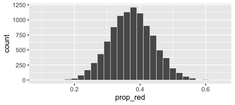
```

![](slide_deck_files/figure-html/unnamed-chunk-48-1.png)

???
If we visualize the proportion of red variable, we can see how the
sample statistic varies from one sample to another for samples of size 50.
---

## Shifting focus

### What about if all we had was the one sample of balls (not the whole bowl)?

```r
jennys_sample %>% count(color)
```

```
# A tibble: 2 x 2
  color     n
* <chr> <int>
1 red      16
2 white    34
```

???
- In reality, we don't usually have the population of interest like we did here
with the `bowl` tibble.
- Rather we have only one sample and would like to understand the variability
we might expect from one sample to another.
--

### How could we use this sample to make a guess about the sampling variability from other samples?

???
- So how can we do this?
---

## Building up to statistical inference!

```r
library(infer)
jennys_sample %>%
  specify(formula = color ~ NULL, success = "red")
```

```
Response: color (factor)
# A tibble: 50 x 1
  color
  <fct>
1 white
2 white
3 white
4 white
5 red  
# … with 45 more rows
```

???
- The infer package provides a way for us to do just this.
- We'll formalize the different functions in a bit but I want to first walk
through our example to help you get a feel for the syntax.
- First we specify that we are interested in looking for red balls with
a response variable set to color.

---

## Bootstrapping?

```r
library(infer)
(bootstrap_samples <- jennys_sample %>%
  specify(formula = color ~ NULL, success = "red") %>%
  generate(reps = 5, type = "bootstrap"))
```

```
Response: color (factor)
# A tibble: 250 x 2
# Groups:   replicate [5]
  replicate color
      <int> <fct>
1         1 red  
2         1 white
3         1 white
4         1 white
5         1 white
# … with 245 more rows
```

???
- We can use sampling with replacement from the color variable to create
bootstrap samples from our original sample of Jenny's.
- Five is chosen for the number of reps here just to help you see what is
going on initially.

---

## What does `bootstrap_samples` represent?

- Remember we assumed that all we had was the original sample of 19 red and 31 white to start.
--

- Hope each of the five sample selections in `bootstrap_samples` is similar to:

???
One way I like to think about bootstrap sampling is that each bootstrap sample
is an attempt to guess at what the population might look like, using the 
original single sample as a guide.

---

## Bootstrap statistics

```r
jennys_sample %>%
  specify(formula = color ~ NULL, success = "red") %>%
  generate(reps = 5, type = "bootstrap") %>%
  calculate(stat = "prop")
```

```
# A tibble: 5 x 2
  replicate  stat
*     <int> <dbl>
1         1  0.4 
2         2  0.32
3         3  0.3 
4         4  0.24
5         5  0.44
```

???
After collecting the samples, we last calculate the proportion of red balls
in each bootstrap sample to obtain five different bootstrap statistics.

---

## Do 10,000 reps to get a better sense for variability

### Just as we did with the sampling distribution

```r
bootstrap_stats <- jennys_sample %>%
  specify(formula = color ~ NULL, success = "red") %>%
  generate(reps = 10000, type = "bootstrap") %>%
  calculate(stat = "prop")
```

???
- Lastly, we can go a step further and repeat this bootstrapping process many
times, say ten thousand.
- And then visualize it which we'll see next.

---

### The bootstrap distribution

![](slide_deck_files/figure-html/unnamed-chunk-54-1.png)

???
- I've added in some bars here corresponding to the mean of the distribution
as well as one standard deviation in both directions.
- This can provide a way to get a sense for sampling variability using
only a single sample.
--

### The sampling distribution

![](slide_deck_files/figure-html/unnamed-chunk-55-1.png)

???
- If you compare this to the actual sampling distribution we calculated before,
you can see that the variation in the two plots is similar.
- Thus, assuming you have a random sample from the population to start (and it
is of reasonable size---whatever that may mean for your problem), bootstrapping
can be a nice way to estimate the variability from one sample to another based
on your statistic of interest.

---

## Get a confidence interval

```r
get_ci(bootstrap_stats, level = 0.95)
```

```
# A tibble: 1 x 2
  lower_ci upper_ci
     <dbl>    <dbl>
1      0.2     0.44
```

- We are 95% "confident" the true proportion of red balls in the hopper/bowl is
between 0.2 and 0.44.

???
- The infer package also includes a get_ci function, which you can use
to return the appropriate percentiles of the bootstrap distribution
corresponding to the level given.

--
***

- In the population:

```r
mean(bowl$color == "red")
```

```
[1] 0.375
```

???
- In this case, we expect about 95 confidence intervals out of 100 to include
the true value from the population and that's why we put confident in quotes.
- As a check since we know the population, we can calculate this proportion.
- Here we see that Jenny's sample would be one of the 95% of intervals that
includes the true population parameter of red balls.
---

## {infer} verbs

???
- You've seen these verbs now via example but I'd like to walk through them
again now with a diagram.
- First, you specify which columns you'd like to work with. You've seen so far
only choosing one variable but you'll see soon that you can select a response
variable and an explanatory variable.
- Then, you can generate bootstrap samples.
- And calculate the appropriate statistic of interest from each sample.
- Looking at the standard deviation of these statistics provides as estimate
for the standard error denoted as SE here.

---

## {infer} verbs

???
- The infer package was designed to also help with hypothesis testing.
- There is only one additional function there with `hypothesize()`.
- That allows you to denote what type of hypothesis test you are wanting to
perform as well as any other null values as needed.
- The `visualize()` function is a wrapper around ggplot2 to provide a quick
way to look at the statistics that have been produced.
- We'll see this further in our next example.

---

# Statistical Inference

<br>

.footnote[{infer} hex sticker designs kindly created by [Thomas Mock](https://www.linkedin.com/in/jthomasmock/)]

???
Thomas Mock was kind enough to produce a few different options for the
{infer} package hex sticker. My personal favorite is here with the gnome
learning about the unknown mu parameter from being in the fir tree.

---

# Research Question

If you see someone else yawn, are you more likely to yawn?

In an episode of the show *Mythbusters*, they tested the myth that yawning is contagious.

--
- 50 adults who thought they were being considered for an appearance on the show.

- Each participant was interviewed individually by a show recruiter ("confederate") who either yawned or did not.

- Participants then sat by themselves in a large van and were asked to wait.

- While in the van, the Mythbusters watched to see if the unaware participants yawned.

???
- Next, I'd walk through another example that lends itself nicely to a hypothesis
testing framework.
- The TV show Mythbusters wanted to test if yawning is contagious.
- They selected 50 adults and split them into two groups.
- Some were shown a yawn and some weren't.
- They they observed whether each participant also yawned.

---

### Data

- `group`
  - 34 saw the confederate yawn (`seed`)
  - 16 did not see the confederate yawn (`control`)
- `yawn`
  - `yes` - participant yawned
  - `no` - participant did not yawn

```r
library(moderndive)
mythbusters_yawn %>% slice(c(1, 3, 6, 19))
```

```
# A tibble: 4 x 3
   subj group   yawn 
  <int> <chr>   <chr>
1     1 seed    yes  
2     3 seed    no   
3     6 control no   
4    19 control yes  
```

???
In the moderndive package, we've included a tibble based on the data presented.
Here are what a few rows of that data looks like.

---

# Results

```r
library(janitor)
mythbusters_yawn %>%
  tabyl(group, yawn) %>%
  adorn_percentages() %>%
  adorn_pct_formatting() %>%
  adorn_ns()
```

```
   group         no        yes
 control 75.0% (12) 25.0%  (4)
    seed 70.6% (24) 29.4% (10)
```

???
- The janitor package provides some tools for looking at the table of yawn versus
group.
- We can see that those who were shown a yawn tended to also yawn more than
those that weren't shown a yawn.
---

## *Finding: CONFIRMED*

> "Though that's not an enormous increase, since they tested 50 people in the field, the gap was still wide enough for the MythBusters to confirm that yawning is indeed contagious." <sup>1</sup>

.footnote[
[1] http://www.discovery.com/tv-shows/mythbusters/mythbusters-database/yawning-contagious/]

???
Mythbusters said this statement on the show. Do you think they did the 
hypothesis test needed to check to see if that claim is appropriate?
---

## Really? Let's formally check this

- State the hypotheses

<br>

Null hypothesis:

> There is no difference between the seed and control groups in the proportion of people who yawned.

Alternative hypothesis (directional):

> More people (relatively) yawned in the seed group than in the control group.

---

## Test the hypothesis

**QUIZ**: Which type of hypothesis test would you conduct here?

- A. Independent samples t-test  
- B. Two proportion test  
- C. Chi-square Goodness of Fit  
- D. Analysis of Variance

---

## Two proportion test

`$$H_0: p_{seed} - p_{control} = 0$$`

`$$H_A: p_{seed} - p_{control} > 0$$`

---

## The observed difference

```r
library(infer)
obs_diff <- mythbusters_yawn %>% 
  specify(yawn ~ group, success = "yes") %>%
  calculate(
    stat = "diff in props",
    order = c("seed", "control")
  )
obs_diff
```

```
# A tibble: 1 x 1
    stat
   <dbl>
1 0.0441
```

???
We've added a shortcut into infer for calculating the observed statistic using
just specify and calculate. We'll add more verbs to this when we get to doing
the hypothesis test with infer.

---
class: middle, center

## Is this difference *meaningful*?

## Different question:

## Is this difference *significant*?

---

# Modeling the null hypothesis

If...

<br>

&emsp;&emsp; `$H_0: p_{seed} = p_{control}$` &emsp;&emsp;

<br>

is true, then whether or not the participant saw someone else yawn does not matter.

<br>

In other words, there is no association between exposure and yawning.

???
We can test for independence between the group and yawn variables.

---
class: center, middle

![](http://directorsnotes.com/wp-content/uploads/2011/11/another_earth_03.jpg)
???
One way to think about this framework of hypothesis testing is by
creating parallel universes where the null hypothesis is true and then
see where what we observed falls in relation to that.

---

.pull-left[
### Original universe
<table>
 <thead>
  <tr>
   <th style="text-align:right;"> subj </th>
   <th style="text-align:left;"> group </th>
   <th style="text-align:left;"> yawn </th>
  </tr>
 </thead>
<tbody>
  <tr>
   <td style="text-align:right;"> 1 </td>
   <td style="text-align:left;"> seed </td>
   <td style="text-align:left;"> yes </td>
  </tr>
  <tr>
   <td style="text-align:right;"> 2 </td>
   <td style="text-align:left;"> control </td>
   <td style="text-align:left;"> yes </td>
  </tr>
  <tr>
   <td style="text-align:right;"> 3 </td>
   <td style="text-align:left;"> seed </td>
   <td style="text-align:left;"> no </td>
  </tr>
  <tr>
   <td style="text-align:right;"> 4 </td>
   <td style="text-align:left;"> seed </td>
   <td style="text-align:left;"> yes </td>
  </tr>
  <tr>
   <td style="text-align:right;"> 5 </td>
   <td style="text-align:left;"> seed </td>
   <td style="text-align:left;"> no </td>
  </tr>
  <tr>
   <td style="text-align:right;"> 6 </td>
   <td style="text-align:left;"> control </td>
   <td style="text-align:left;"> no </td>
  </tr>
  <tr>
   <td style="text-align:right;"> 15 </td>
   <td style="text-align:left;"> seed </td>
   <td style="text-align:left;"> no </td>
  </tr>
  <tr>
   <td style="text-align:right;"> 16 </td>
   <td style="text-align:left;"> seed </td>
   <td style="text-align:left;"> no </td>
  </tr>
  <tr>
   <td style="text-align:right;"> 17 </td>
   <td style="text-align:left;"> seed </td>
   <td style="text-align:left;"> no </td>
  </tr>
  <tr>
   <td style="text-align:right;"> 18 </td>
   <td style="text-align:left;"> seed </td>
   <td style="text-align:left;"> no </td>
  </tr>
  <tr>
   <td style="text-align:right;"> 19 </td>
   <td style="text-align:left;"> control </td>
   <td style="text-align:left;"> yes </td>
  </tr>
  <tr>
   <td style="text-align:right;"> 20 </td>
   <td style="text-align:left;"> seed </td>
   <td style="text-align:left;"> no </td>
  </tr>
</tbody>
</table>

```
   group no yes Total
 control 12   4    16
    seed 24  10    34
   Total 36  14    50
```
]

???
Our original universe looks like this.

.pull-right[
### Parallel universe
<table>
 <thead>
  <tr>
   <th style="text-align:right;"> subj </th>
   <th style="text-align:left;"> group </th>
   <th style="text-align:left;"> alt_yawn </th>
  </tr>
 </thead>
<tbody>
  <tr>
   <td style="text-align:right;"> 1 </td>
   <td style="text-align:left;"> seed </td>
   <td style="text-align:left;"> yes </td>
  </tr>
  <tr>
   <td style="text-align:right;"> 2 </td>
   <td style="text-align:left;"> control </td>
   <td style="text-align:left;"> no </td>
  </tr>
  <tr>
   <td style="text-align:right;"> 3 </td>
   <td style="text-align:left;"> seed </td>
   <td style="text-align:left;"> no </td>
  </tr>
  <tr>
   <td style="text-align:right;"> 4 </td>
   <td style="text-align:left;"> seed </td>
   <td style="text-align:left;"> no </td>
  </tr>
  <tr>
   <td style="text-align:right;"> 5 </td>
   <td style="text-align:left;"> seed </td>
   <td style="text-align:left;"> yes </td>
  </tr>
  <tr>
   <td style="text-align:right;"> 6 </td>
   <td style="text-align:left;"> control </td>
   <td style="text-align:left;"> yes </td>
  </tr>
  <tr>
   <td style="text-align:right;"> 15 </td>
   <td style="text-align:left;"> seed </td>
   <td style="text-align:left;"> no </td>
  </tr>
  <tr>
   <td style="text-align:right;"> 16 </td>
   <td style="text-align:left;"> seed </td>
   <td style="text-align:left;"> no </td>
  </tr>
  <tr>
   <td style="text-align:right;"> 17 </td>
   <td style="text-align:left;"> seed </td>
   <td style="text-align:left;"> no </td>
  </tr>
  <tr>
   <td style="text-align:right;"> 18 </td>
   <td style="text-align:left;"> seed </td>
   <td style="text-align:left;"> yes </td>
  </tr>
  <tr>
   <td style="text-align:right;"> 19 </td>
   <td style="text-align:left;"> control </td>
   <td style="text-align:left;"> no </td>
  </tr>
  <tr>
   <td style="text-align:right;"> 20 </td>
   <td style="text-align:left;"> seed </td>
   <td style="text-align:left;"> yes </td>
  </tr>
</tbody>
</table>

```
   group no yes Total
 control 10   6    16
    seed 26   8    34
   Total 36  14    50
```
]

???
One parallel universe looks like this. Notice that the overall Totals in the 
table at the bottom stays the same, but the values of the response variable have
been shuffled.

---

# 1000 parallel universes

.pull-left[
<table>
 <thead>
  <tr>
   <th style="text-align:right;"> replicate </th>
   <th style="text-align:right;"> stat </th>
  </tr>
 </thead>
<tbody>
  <tr>
   <td style="text-align:right;"> 1 </td>
   <td style="text-align:right;"> 0.22794 </td>
  </tr>
  <tr>
   <td style="text-align:right;"> 2 </td>
   <td style="text-align:right;"> 0.41176 </td>
  </tr>
  <tr>
   <td style="text-align:right;"> 3 </td>
   <td style="text-align:right;"> 0.04412 </td>
  </tr>
  <tr>
   <td style="text-align:right;"> 4 </td>
   <td style="text-align:right;"> 0.04412 </td>
  </tr>
  <tr>
   <td style="text-align:right;"> 5 </td>
   <td style="text-align:right;"> -0.04779 </td>
  </tr>
  <tr>
   <td style="text-align:right;"> 6 </td>
   <td style="text-align:right;"> 0.13603 </td>
  </tr>
  <tr>
   <td style="text-align:right;"> 7 </td>
   <td style="text-align:right;"> -0.23162 </td>
  </tr>
  <tr>
   <td style="text-align:right;"> 8 </td>
   <td style="text-align:right;"> 0.22794 </td>
  </tr>
  <tr>
   <td style="text-align:right;"> 9 </td>
   <td style="text-align:right;"> -0.04779 </td>
  </tr>
  <tr>
   <td style="text-align:right;"> 10 </td>
   <td style="text-align:right;"> 0.04412 </td>
  </tr>
  <tr>
   <td style="text-align:right;"> 11 </td>
   <td style="text-align:right;"> 0.13603 </td>
  </tr>
  <tr>
   <td style="text-align:right;"> 12 </td>
   <td style="text-align:right;"> 0.04412 </td>
  </tr>
  <tr>
   <td style="text-align:right;"> 13 </td>
   <td style="text-align:right;"> 0.04412 </td>
  </tr>
  <tr>
   <td style="text-align:right;"> 14 </td>
   <td style="text-align:right;"> -0.04779 </td>
  </tr>
  <tr>
   <td style="text-align:right;"> 15 </td>
   <td style="text-align:right;"> -0.13971 </td>
  </tr>
</tbody>
</table>
]

.pull-right[
<table>
 <thead>
  <tr>
   <th style="text-align:right;"> replicate </th>
   <th style="text-align:right;"> stat </th>
  </tr>
 </thead>
<tbody>
  <tr>
   <td style="text-align:right;"> 986 </td>
   <td style="text-align:right;"> 0.04412 </td>
  </tr>
  <tr>
   <td style="text-align:right;"> 987 </td>
   <td style="text-align:right;"> -0.13971 </td>
  </tr>
  <tr>
   <td style="text-align:right;"> 988 </td>
   <td style="text-align:right;"> 0.04412 </td>
  </tr>
  <tr>
   <td style="text-align:right;"> 989 </td>
   <td style="text-align:right;"> -0.23162 </td>
  </tr>
  <tr>
   <td style="text-align:right;"> 990 </td>
   <td style="text-align:right;"> -0.04779 </td>
  </tr>
  <tr>
   <td style="text-align:right;"> 991 </td>
   <td style="text-align:right;"> -0.13971 </td>
  </tr>
  <tr>
   <td style="text-align:right;"> 992 </td>
   <td style="text-align:right;"> -0.13971 </td>
  </tr>
  <tr>
   <td style="text-align:right;"> 993 </td>
   <td style="text-align:right;"> -0.13971 </td>
  </tr>
  <tr>
   <td style="text-align:right;"> 994 </td>
   <td style="text-align:right;"> 0.04412 </td>
  </tr>
  <tr>
   <td style="text-align:right;"> 995 </td>
   <td style="text-align:right;"> -0.13971 </td>
  </tr>
  <tr>
   <td style="text-align:right;"> 996 </td>
   <td style="text-align:right;"> -0.23162 </td>
  </tr>
  <tr>
   <td style="text-align:right;"> 997 </td>
   <td style="text-align:right;"> 0.13603 </td>
  </tr>
  <tr>
   <td style="text-align:right;"> 998 </td>
   <td style="text-align:right;"> -0.04779 </td>
  </tr>
  <tr>
   <td style="text-align:right;"> 999 </td>
   <td style="text-align:right;"> 0.04412 </td>
  </tr>
  <tr>
   <td style="text-align:right;"> 1000 </td>
   <td style="text-align:right;"> 0.04412 </td>
  </tr>
</tbody>
</table>
]

???
We can next think about 1000 such parallel universes as well as the difference
in proportions for each of those replicates.

---
## The parallel universe distribution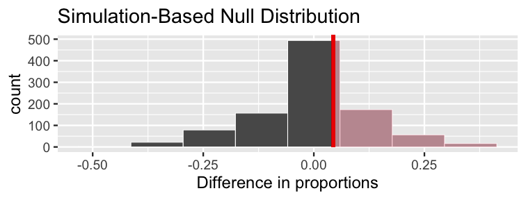

![](slide_deck_files/figure-html/unnamed-chunk-65-1.png)

The distribution of 1000 differences in proportions, if the null hypothesis were *true* and yawning was not contagious.

???
It's always a little weird shading a histogram but you can see that around
40-50% of the values in this null distribution are greater than what we 
observed.

---
## Calculating the p-value

<br>

The shaded proportion is the p-value!

```r
null_distn %>% 
  get_p_value(obs_stat = obs_diff, direction = "right")
```

```
# A tibble: 1 x 1
  p_value
    <dbl>
1   0.493
```

???
- We can calculate this value directly using the get_p_value function from infer.
- This determines the proportion of statistics that are as extreme or more
extreme than what was observed in our sample.

---
class: middle, center
layout: false

## There is Only One Test!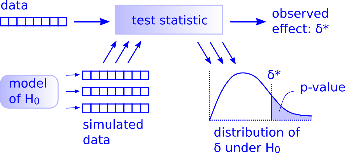

[![Only One Test](images/downey.png)](http://allendowney.blogspot.com/2016/06/there-is-still-only-one-test.html)

???
This framework for thinking about hypothesis testing was inspired by
Allen Downey and his "There is Only One Test!" blogpost. If you click on the
diagram here it will send you to this webpage.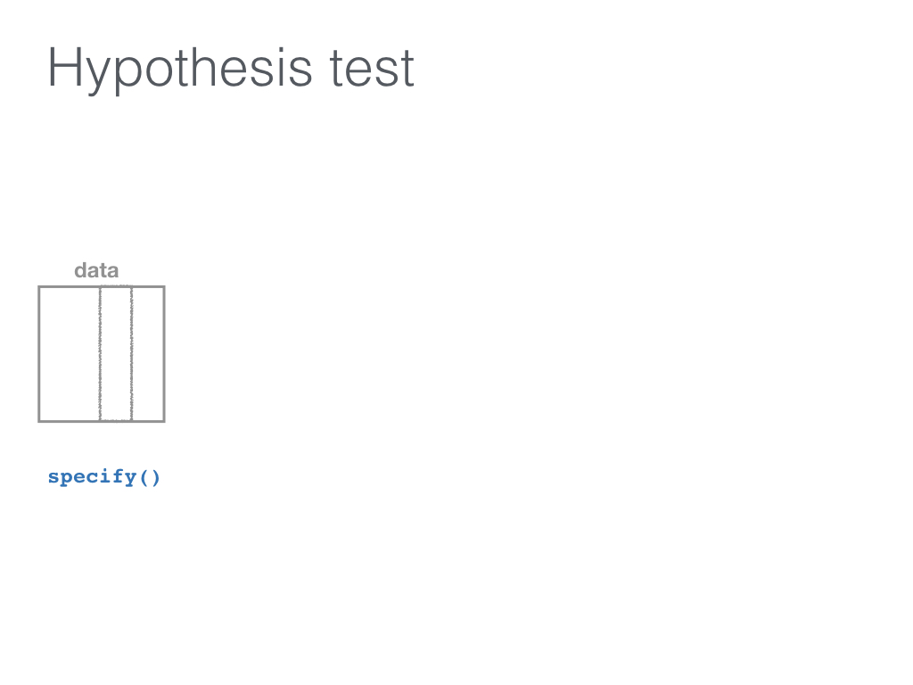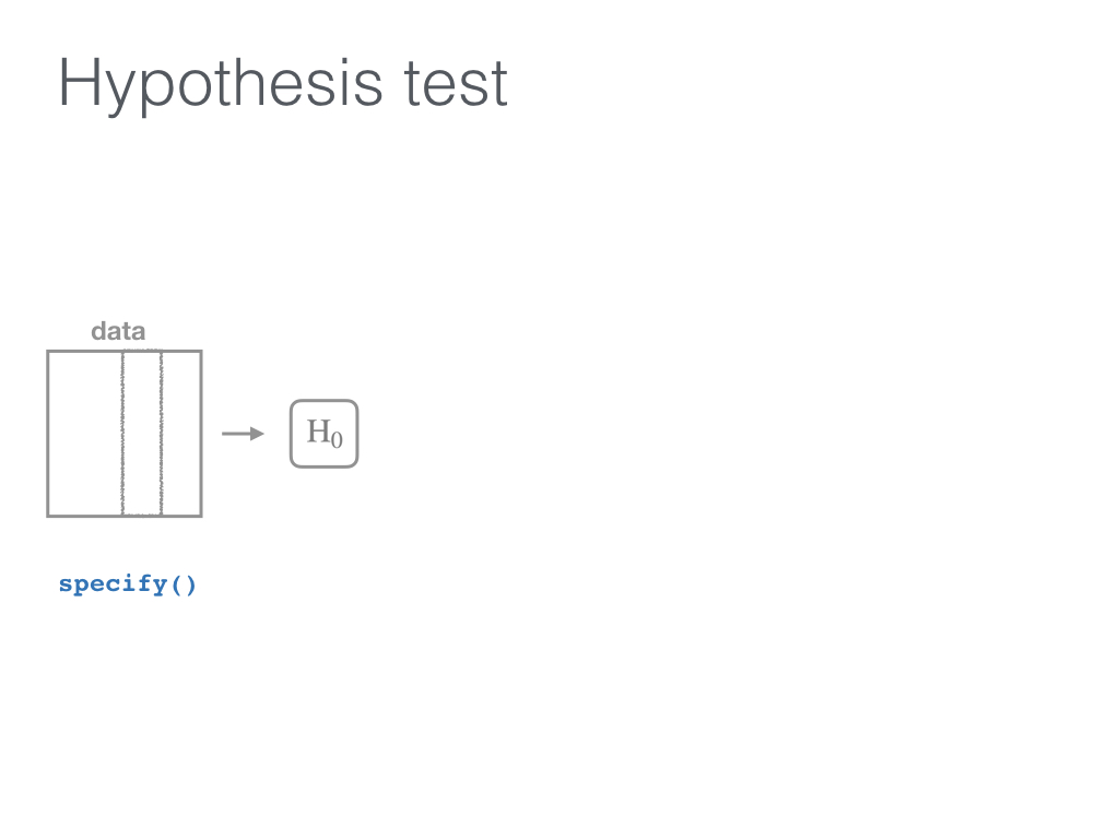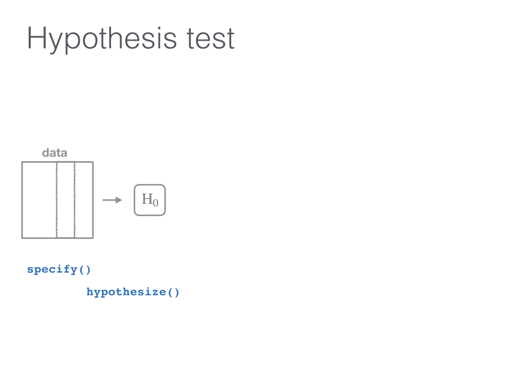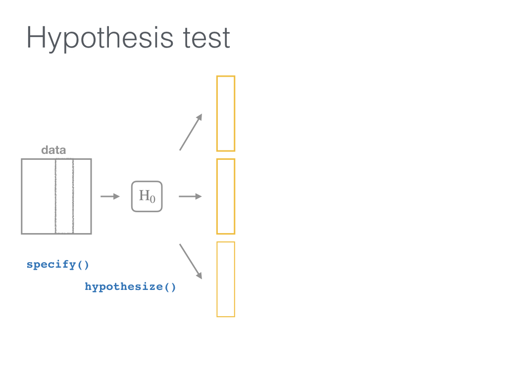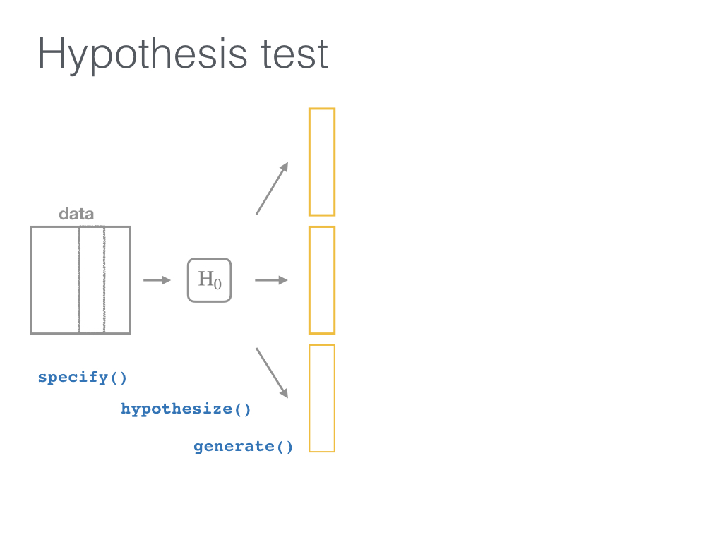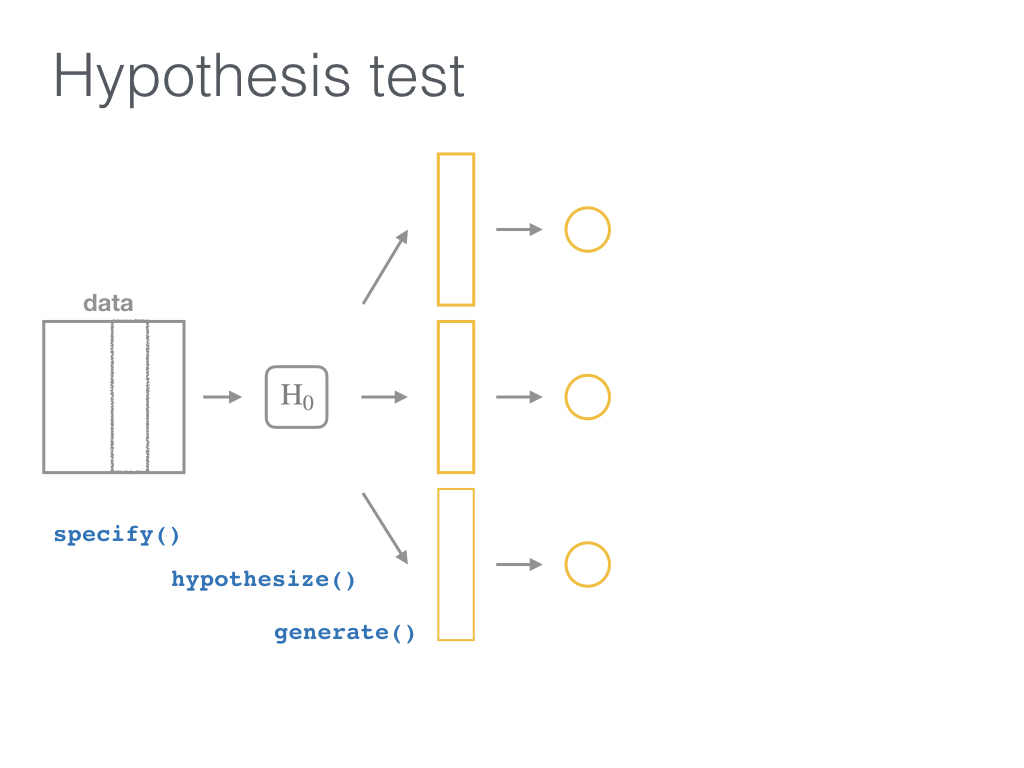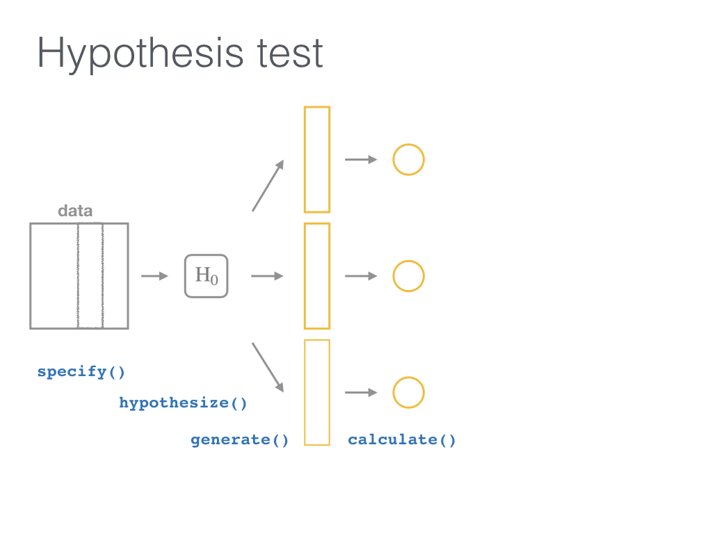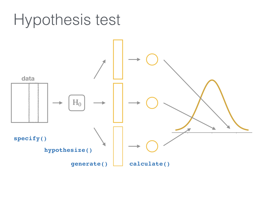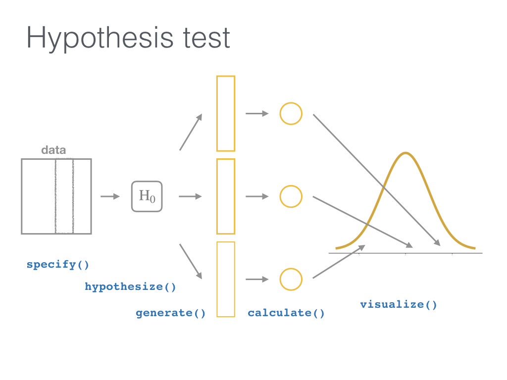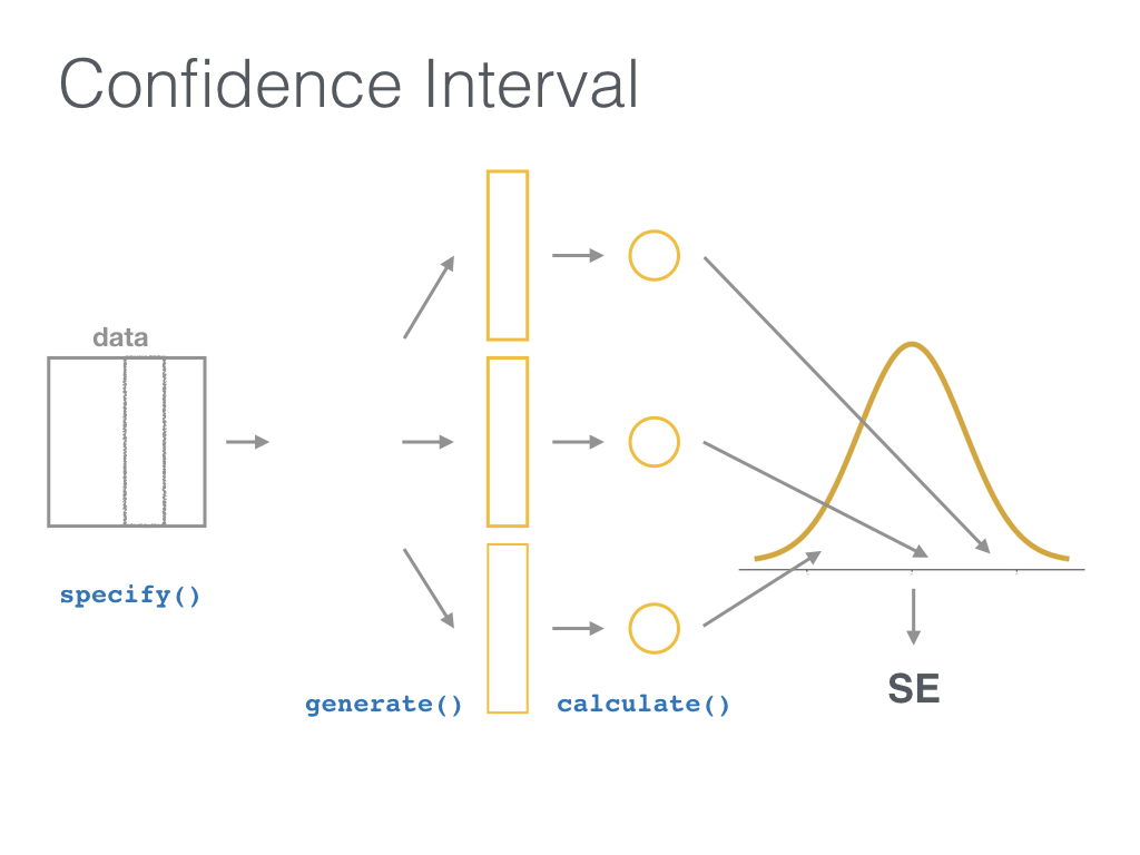

---

![](images/infer.073.jpeg)

---

![](images/infer.074.jpeg)

---

![](images/infer.075.jpeg)

---

![](images/infer.076.jpeg)

---

![](images/infer.077.jpeg)

---

![](images/infer.078.jpeg)

---

![](images/infer.079.jpeg)

---

![](images/infer.080.jpeg)

---

![](images/infer.081.jpeg)

---

![](images/infer.082.jpeg)

---

![](images/infer.084.jpeg)

---

## {infer}

Five main functions:

- `specify()`
- `hypothesize()`
- `generate()`
- `calculate()`
- `visualize()`

---

## {infer}
<small>
- `specify()` the response and explanatory variables (`y ~ x`)
- `hypothesize()` what the null hypothesis is (here, `independence` of `y` and `x`)
- `generate()` new samples from parallel universes under the null hypothesis model:
    - <small>Resample from our original data <u>without replacement</u>, each time shuffling the `group` (`type = "permute"`)</small>
    - <small>Do this <u>a ton of times</u> (`reps = 1000`)</small>
- `calculate()` the statistic (`stat = "diff in props"`) for each of the `reps`
</small>

???
This slide gives you more details on what each step in the process looks like
for this example.

---

## {infer} example

```r
set.seed(8)
null_distn <- mythbusters_yawn %>%
  specify(
    formula = yawn ~ group, 
    success = "yes"
  ) %>%
  hypothesize(null = "independence") %>%
  generate(reps = 1000, type = "permute") %>%
  calculate(
    stat = "diff in props", 
    order = c("seed", "control")
  )
```

???
The infer pipeline is verbose but it is designed to help beginners understand
simulation-based inference via the code written. It helps remind them of how
the problem is set up as well as the steps in Allen Downey's framework.

---

## Visualize the null distribution

- `visualize()` the distribution of the `stat` <br> (here, `diff in props`)

```r
null_distn %>%
  visualize(bins = 8) +
  shade_p_value(obs_stat = obs_diff, direction = "right")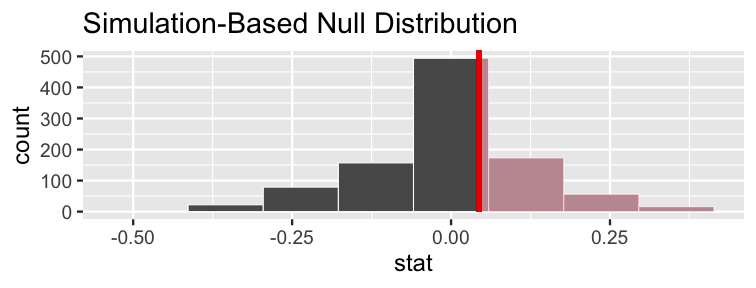
```

![](slide_deck_files/figure-html/unnamed-chunk-69-1.png)

???
Lastly, we can visualize and shade in the p-value to get a sense for its value
as well as a conceptual understanding of what it represents for this problem.

---

## Classical inference

Rely on theory to tell us what the null distribution looks like.

```r
obs_z <- mythbusters_yawn %>%
  specify(yawn ~ group, success = "yes") %>%
  calculate(stat = "z", order = c("seed", "control"))

mythbusters_yawn %>%
  specify(yawn ~ group, success = "yes") %>%
  hypothesize(null = "independence") %>%
  # generate() is not needed since we are not simulating
  calculate(stat = "z", order = c("seed", "control")) %>%
  visualize(method = "theoretical") +
  shade_p_value(obs_stat = obs_z, direction = "right")
```

???
- infer also works for many of the common traditional classical inference
techniques like performing a z test here.
- The syntax is much the same except now we are calculating a z statistic
and we don't need to use generate since the normal distribution will be
used directly.

---

## Classical inference

```
Warning: Check to make sure the conditions have been met for the
theoretical method. {infer} currently does not check these for
you.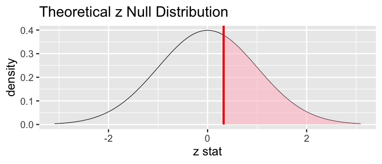
```

![](slide_deck_files/figure-html/unnamed-chunk-72-1.png)

???
infer also gives a warning here that the assumptions behind a traditional
hypothesis test such as sample size and independence of observations have
not been checked.

---

# Simulation-based vs Classical (`stat = "z"`)

```r
mythbusters_yawn %>%
  specify(yawn ~ group, success = "yes") %>%
  hypothesize(null = "independence") %>%
  generate(reps = 1000, type = "permute") %>%
  calculate(stat = "z", order = c("seed", "control")) %>%
  visualize(method = "both", bins = 8) + 
  shade_p_value(obs_stat = obs_z, direction = "right")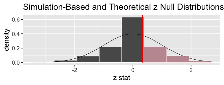
```

![](slide_deck_files/figure-html/unnamed-chunk-73-1.png)

???
Lastly, you can do both simulation and classical types of inference at the same
time using `visualize(method = "both)`.

---

## More info and resources

- https://infer.tidymodels.org/
  - Many examples under Articles
  - Discussed in [www.ModernDive.com](https://www.ModernDive.com)
      - [Sign up](http://eepurl.com/cBkItf) to the mailing list for updates
- [Learn the tidyverse](https://www.tidyverse.org/learn/)

---

## Any further questions?

- Slides created via the R package [xaringan](https://github.com/yihui/xaringan) by Yihui Xie
- Slides' source code at <https://github.com/ismayc/talks/>
- R code from throughout the slides as an R script as [slide_code.R](https://raw.githubusercontent.com/ismayc/talks/master/csp-2021/slide_code.R)

---

# Thanks!

.pull-left[
  [<svg style="height:0.8em;top:.04em;position:relative;" viewBox="0 0 512 512"><path d="M459.37 151.716c.325 4.548.325 9.097.325 13.645 0 138.72-105.583 298.558-298.558 298.558-59.452 0-114.68-17.219-161.137-47.106 8.447.974 16.568 1.299 25.34 1.299 49.055 0 94.213-16.568 130.274-44.832-46.132-.975-84.792-31.188-98.112-72.772 6.498.974 12.995 1.624 19.818 1.624 9.421 0 18.843-1.3 27.614-3.573-48.081-9.747-84.143-51.98-84.143-102.985v-1.299c13.969 7.797 30.214 12.67 47.431 13.319-28.264-18.843-46.781-51.005-46.781-87.391 0-19.492 5.197-37.36 14.294-52.954 51.655 63.675 129.3 105.258 216.365 109.807-1.624-7.797-2.599-15.918-2.599-24.04 0-57.828 46.782-104.934 104.934-104.934 30.213 0 57.502 12.67 76.67 33.137 23.715-4.548 46.456-13.32 66.599-25.34-7.798 24.366-24.366 44.833-46.132 57.827 21.117-2.273 41.584-8.122 60.426-16.243-14.292 20.791-32.161 39.308-52.628 54.253z"/></svg> @datapointier](http://twitter.com/datapointier)  
  [<svg style="height:0.8em;top:.04em;position:relative;" viewBox="0 0 496 512"><path d="M165.9 397.4c0 2-2.3 3.6-5.2 3.6-3.3.3-5.6-1.3-5.6-3.6 0-2 2.3-3.6 5.2-3.6 3-.3 5.6 1.3 5.6 3.6zm-31.1-4.5c-.7 2 1.3 4.3 4.3 4.9 2.6 1 5.6 0 6.2-2s-1.3-4.3-4.3-5.2c-2.6-.7-5.5.3-6.2 2.3zm44.2-1.7c-2.9.7-4.9 2.6-4.6 4.9.3 2 2.9 3.3 5.9 2.6 2.9-.7 4.9-2.6 4.6-4.6-.3-1.9-3-3.2-5.9-2.9zM244.8 8C106.1 8 0 113.3 0 252c0 110.9 69.8 205.8 169.5 239.2 12.8 2.3 17.3-5.6 17.3-12.1 0-6.2-.3-40.4-.3-61.4 0 0-70 15-84.7-29.8 0 0-11.4-29.1-27.8-36.6 0 0-22.9-15.7 1.6-15.4 0 0 24.9 2 38.6 25.8 21.9 38.6 58.6 27.5 72.9 20.9 2.3-16 8.8-27.1 16-33.7-55.9-6.2-112.3-14.3-112.3-110.5 0-27.5 7.6-41.3 23.6-58.9-2.6-6.5-11.1-33.3 2.6-67.9 20.9-6.5 69 27 69 27 20-5.6 41.5-8.5 62.8-8.5s42.8 2.9 62.8 8.5c0 0 48.1-33.6 69-27 13.7 34.7 5.2 61.4 2.6 67.9 16 17.7 25.8 31.5 25.8 58.9 0 96.5-58.9 104.2-114.8 110.5 9.2 7.9 17 22.9 17 46.4 0 33.7-.3 75.4-.3 83.6 0 6.5 4.6 14.4 17.3 12.1C428.2 457.8 496 362.9 496 252 496 113.3 383.5 8 244.8 8zM97.2 352.9c-1.3 1-1 3.3.7 5.2 1.6 1.6 3.9 2.3 5.2 1 1.3-1 1-3.3-.7-5.2-1.6-1.6-3.9-2.3-5.2-1zm-10.8-8.1c-.7 1.3.3 2.9 2.3 3.9 1.6 1 3.6.7 4.3-.7.7-1.3-.3-2.9-2.3-3.9-2-.6-3.6-.3-4.3.7zm32.4 35.6c-1.6 1.3-1 4.3 1.3 6.2 2.3 2.3 5.2 2.6 6.5 1 1.3-1.3.7-4.3-1.3-6.2-2.2-2.3-5.2-2.6-6.5-1zm-11.4-14.7c-1.6 1-1.6 3.6 0 5.9 1.6 2.3 4.3 3.3 5.6 2.3 1.6-1.3 1.6-3.9 0-6.2-1.4-2.3-4-3.3-5.6-2z"/></svg> @jminnier](http://github.com/jminnier)  
  [<svg style="height:0.8em;top:.04em;position:relative;" viewBox="0 0 512 512"><path d="M326.612 185.391c59.747 59.809 58.927 155.698.36 214.59-.11.12-.24.25-.36.37l-67.2 67.2c-59.27 59.27-155.699 59.262-214.96 0-59.27-59.26-59.27-155.7 0-214.96l37.106-37.106c9.84-9.84 26.786-3.3 27.294 10.606.648 17.722 3.826 35.527 9.69 52.721 1.986 5.822.567 12.262-3.783 16.612l-13.087 13.087c-28.026 28.026-28.905 73.66-1.155 101.96 28.024 28.579 74.086 28.749 102.325.51l67.2-67.19c28.191-28.191 28.073-73.757 0-101.83-3.701-3.694-7.429-6.564-10.341-8.569a16.037 16.037 0 0 1-6.947-12.606c-.396-10.567 3.348-21.456 11.698-29.806l21.054-21.055c5.521-5.521 14.182-6.199 20.584-1.731a152.482 152.482 0 0 1 20.522 17.197zM467.547 44.449c-59.261-59.262-155.69-59.27-214.96 0l-67.2 67.2c-.12.12-.25.25-.36.37-58.566 58.892-59.387 154.781.36 214.59a152.454 152.454 0 0 0 20.521 17.196c6.402 4.468 15.064 3.789 20.584-1.731l21.054-21.055c8.35-8.35 12.094-19.239 11.698-29.806a16.037 16.037 0 0 0-6.947-12.606c-2.912-2.005-6.64-4.875-10.341-8.569-28.073-28.073-28.191-73.639 0-101.83l67.2-67.19c28.239-28.239 74.3-28.069 102.325.51 27.75 28.3 26.872 73.934-1.155 101.96l-13.087 13.087c-4.35 4.35-5.769 10.79-3.783 16.612 5.864 17.194 9.042 34.999 9.69 52.721.509 13.906 17.454 20.446 27.294 10.606l37.106-37.106c59.271-59.259 59.271-155.699.001-214.959z"/></svg> jessicaminnier.com](https:/jessicaminnier.com)  

]

.pull-right[
  [<svg style="height:0.8em;top:.04em;position:relative;" viewBox="0 0 512 512"><path d="M459.37 151.716c.325 4.548.325 9.097.325 13.645 0 138.72-105.583 298.558-298.558 298.558-59.452 0-114.68-17.219-161.137-47.106 8.447.974 16.568 1.299 25.34 1.299 49.055 0 94.213-16.568 130.274-44.832-46.132-.975-84.792-31.188-98.112-72.772 6.498.974 12.995 1.624 19.818 1.624 9.421 0 18.843-1.3 27.614-3.573-48.081-9.747-84.143-51.98-84.143-102.985v-1.299c13.969 7.797 30.214 12.67 47.431 13.319-28.264-18.843-46.781-51.005-46.781-87.391 0-19.492 5.197-37.36 14.294-52.954 51.655 63.675 129.3 105.258 216.365 109.807-1.624-7.797-2.599-15.918-2.599-24.04 0-57.828 46.782-104.934 104.934-104.934 30.213 0 57.502 12.67 76.67 33.137 23.715-4.548 46.456-13.32 66.599-25.34-7.798 24.366-24.366 44.833-46.132 57.827 21.117-2.273 41.584-8.122 60.426-16.243-14.292 20.791-32.161 39.308-52.628 54.253z"/></svg> @old_man_chester](http://twitter.com/old_man_chester)  
  [<svg style="height:0.8em;top:.04em;position:relative;" viewBox="0 0 496 512"><path d="M165.9 397.4c0 2-2.3 3.6-5.2 3.6-3.3.3-5.6-1.3-5.6-3.6 0-2 2.3-3.6 5.2-3.6 3-.3 5.6 1.3 5.6 3.6zm-31.1-4.5c-.7 2 1.3 4.3 4.3 4.9 2.6 1 5.6 0 6.2-2s-1.3-4.3-4.3-5.2c-2.6-.7-5.5.3-6.2 2.3zm44.2-1.7c-2.9.7-4.9 2.6-4.6 4.9.3 2 2.9 3.3 5.9 2.6 2.9-.7 4.9-2.6 4.6-4.6-.3-1.9-3-3.2-5.9-2.9zM244.8 8C106.1 8 0 113.3 0 252c0 110.9 69.8 205.8 169.5 239.2 12.8 2.3 17.3-5.6 17.3-12.1 0-6.2-.3-40.4-.3-61.4 0 0-70 15-84.7-29.8 0 0-11.4-29.1-27.8-36.6 0 0-22.9-15.7 1.6-15.4 0 0 24.9 2 38.6 25.8 21.9 38.6 58.6 27.5 72.9 20.9 2.3-16 8.8-27.1 16-33.7-55.9-6.2-112.3-14.3-112.3-110.5 0-27.5 7.6-41.3 23.6-58.9-2.6-6.5-11.1-33.3 2.6-67.9 20.9-6.5 69 27 69 27 20-5.6 41.5-8.5 62.8-8.5s42.8 2.9 62.8 8.5c0 0 48.1-33.6 69-27 13.7 34.7 5.2 61.4 2.6 67.9 16 17.7 25.8 31.5 25.8 58.9 0 96.5-58.9 104.2-114.8 110.5 9.2 7.9 17 22.9 17 46.4 0 33.7-.3 75.4-.3 83.6 0 6.5 4.6 14.4 17.3 12.1C428.2 457.8 496 362.9 496 252 496 113.3 383.5 8 244.8 8zM97.2 352.9c-1.3 1-1 3.3.7 5.2 1.6 1.6 3.9 2.3 5.2 1 1.3-1 1-3.3-.7-5.2-1.6-1.6-3.9-2.3-5.2-1zm-10.8-8.1c-.7 1.3.3 2.9 2.3 3.9 1.6 1 3.6.7 4.3-.7.7-1.3-.3-2.9-2.3-3.9-2-.6-3.6-.3-4.3.7zm32.4 35.6c-1.6 1.3-1 4.3 1.3 6.2 2.3 2.3 5.2 2.6 6.5 1 1.3-1.3.7-4.3-1.3-6.2-2.2-2.3-5.2-2.6-6.5-1zm-11.4-14.7c-1.6 1-1.6 3.6 0 5.9 1.6 2.3 4.3 3.3 5.6 2.3 1.6-1.3 1.6-3.9 0-6.2-1.4-2.3-4-3.3-5.6-2z"/></svg> @ismayc](http://github.com/ismayc)  
  [<svg style="height:0.8em;top:.04em;position:relative;" viewBox="0 0 512 512"><path d="M326.612 185.391c59.747 59.809 58.927 155.698.36 214.59-.11.12-.24.25-.36.37l-67.2 67.2c-59.27 59.27-155.699 59.262-214.96 0-59.27-59.26-59.27-155.7 0-214.96l37.106-37.106c9.84-9.84 26.786-3.3 27.294 10.606.648 17.722 3.826 35.527 9.69 52.721 1.986 5.822.567 12.262-3.783 16.612l-13.087 13.087c-28.026 28.026-28.905 73.66-1.155 101.96 28.024 28.579 74.086 28.749 102.325.51l67.2-67.19c28.191-28.191 28.073-73.757 0-101.83-3.701-3.694-7.429-6.564-10.341-8.569a16.037 16.037 0 0 1-6.947-12.606c-.396-10.567 3.348-21.456 11.698-29.806l21.054-21.055c5.521-5.521 14.182-6.199 20.584-1.731a152.482 152.482 0 0 1 20.522 17.197zM467.547 44.449c-59.261-59.262-155.69-59.27-214.96 0l-67.2 67.2c-.12.12-.25.25-.36.37-58.566 58.892-59.387 154.781.36 214.59a152.454 152.454 0 0 0 20.521 17.196c6.402 4.468 15.064 3.789 20.584-1.731l21.054-21.055c8.35-8.35 12.094-19.239 11.698-29.806a16.037 16.037 0 0 0-6.947-12.606c-2.912-2.005-6.64-4.875-10.341-8.569-28.073-28.073-28.191-73.639 0-101.83l67.2-67.19c28.239-28.239 74.3-28.069 102.325.51 27.75 28.3 26.872 73.934-1.155 101.96l-13.087 13.087c-4.35 4.35-5.769 10.79-3.783 16.612 5.864 17.194 9.042 34.999 9.69 52.721.509 13.906 17.454 20.446 27.294 10.606l37.106-37.106c59.271-59.259 59.271-155.699.001-214.959z"/></svg> chester.rbind.io](https://chester.rbind.io)  

]

???
We've also included some tips in the Appendix that follows.

---
class: inverse, center, middle

# Appendix

---

## Freely available information

<center><h2>Statistical Inference via Data Science <br> A ModernDive into R and the Tidyverse</h2></center>

* Webpage: <https://moderndive.com>
* Developmental version: <https://moderndive.netlify.app>
* [GitHub Repo](https://github.com/moderndive/ModernDive_book)
* Please [signup](http://eepurl.com/cBkItf) for our mailing list!

---

## Good practices in RStudio

__Use projects__ ([read this](https://r4ds.had.co.nz/workflow-projects.html))
- Create an RStudio project for each data analysis project
- A project is associated with a directory folder
    + Keep data files there
    + Keep scripts there; edit them, run them in bits or as a whole
    + Save your outputs (plots and cleaned data) there

- Only use relative paths, never absolute paths
    + relative (good): `read_csv("data/mydata.csv")`
    + absolute (bad): 
    
    <code><small>read_csv("/home/yourname/Documents/stuff/mydata.csv")</small></code>
    
---

## Advantages of using RStudio projects

- standardize file paths
- keep everything together
- a whole folder can be shared and run on another computer

---

# Useful keyboard shortcuts

action | mac | windows/linux
---| ---| ---
run code in script | cmd + enter | ctrl + enter 
`<-`| option + - | alt + -
`%>%` | cmd + shift + m | ctrl + shift + m
]

```r
y <- 5
y
```
Now, in the console, press the up arrow.
]

---

## Other keyboard shortcuts: ([see full list](https://support.rstudio.com/hc/en-us/articles/200711853-Keyboard-Shortcuts))

action | mac | windows/linux
---| ---| ---
interrupt currently executing command | esc | esc
in console, go to previously run code | up/down | up/down
keyboard shortcut help | option + shift + k | alt + shift + k