class: center, middle, inverse, title-slide # A Fully Customizable Textbook for Introductory Statistics/Data Science ## USCOTS 2017 Workshop ### Chester Ismay and Albert Y. Kim ### May 17 & 18, 2017 <br><br> Slides at <a href="http://bit.ly/uscots17-slides" class="uri">http://bit.ly/uscots17-slides</a> <br> Supplementary HTML document at <a href="http://bit.ly/uscots17-html" class="uri">http://bit.ly/uscots17-html</a> --- <!-- Write slide link on whiteboard --> <!-----------------------------------------------------------------------------> # Introduction ## Who We Are * [Chester Ismay](https://ismayc.github.io/): Reed College & Pacific University + Email: <chester.ismay@gmail.com> + GitHub: [`ismayc`](https://github.com/ismayc) + Twitter: [`@old_man_chester`](https://twitter.com/old_man_chester) * [Albert Y. Kim](http://rudeboybert.github.io/): Middlebury College + Email: <albert.ys.kim@gmail.com> + GitHub: [`rudeboybert`](https://github.com/rudeboybert) + Twitter: [`@rudeboybert`](https://twitter.com/rudeboybert) --- class: center, middle ## Outline of Workshop [Google Doc at <http://bit.ly/uscots17-agenda>](https://docs.google.com/document/d/12Ai7wxK5OTrIwwrSJQewXHcqpMJ09lB-HkGN3BbShy4/edit?usp=sharing) --- ## Our Textbook <img src="figure/moderndive-logo.png" height="75px"/> * *An Introduction to Statistical and Data Sciences via R* * Webpage: <http://moderndive.com>. [GitHub Repo](https://github.com/ismayc/moderndiver-book) * In you haven't already, please [signup](http://moderndive.us15.list-manage2.com/subscribe?u=87888fab720da90906427a5be&id=0c9e2d1df2) for our mailing list! --- ## Albert's Course (Intro to Statistical & Data Sciences) Available in the supplementary HTML document [here](https://ismayc.github.io/moderndive-workshops/slides/slide_document.html#introduction). * [Webpage](https://rudeboybert.github.io/MATH116/) and [GitHub Repo](https://github.com/rudeboybert/MATH116) * Administrative: + Chief non-econ/bio stats service class at Middlebury + 12 weeks each with 3h "lecture" + 1h "lab" + <u>No prerequisites</u> * Students: + ~24 students/section of all years/backgrounds. Only stats class many will take + Background: Many had AP stats, some with programming + All had laptops that they brought everyday * [Topic List](https://rudeboybert.github.io/MATH116/) + <u>First half is data science</u>: data visualization, manipulation, importing + <u>Second half is intro stats</u>: sampling, hypothesis tests, CI, regression * Evaluation + 10%: weekly problem sets + 10%: engagement + 45%: 3 midterms (last during finals week) + <u>35%: [Final projects](https://rudeboybert.github.io/MATH116/PS/final_project/final_project_outline.html#learning_goals)</u> * Typical Classtime: + First 10-15min: Priming topic, either via slides or <u>chalk talk</u> + Remainder: Students read over text & do <u>Learning Checks</u> in groups and without direct instructor guidance. --- ## Chester's Course (Social Statistics) Available in the supplementary HTML document [here](https://ismayc.github.io/moderndive-workshops/slides/slide_document.html#introduction) * [Webpage at <http://bit.ly/soc-301>](https://ismayc.github.io/soc301_s2017/) and [GitHub Repo](https://github.com/ismayc/soc301_s2017) * Administrative: + Chief stats service class for sociology/criminal justice + An option take to fulfill the Pacific U. math requirement + 14 weeks, meeting on Tues & Thurs for 95 minutes + <u>No prerequisites</u> * Students: + 26 students of all years/backgrounds. Only stats class many will take + Background: 3 had AP stats, zero with programming + All had laptops that they brought everyday * [Course Schedule](https://ismayc.github.io/soc301_s2017/schedule/) + <u>First half is data science</u>: data visualization, wrangling, importing + <u>Second half is intro stats</u>: sampling, testing, CI * [Evaluation](https://ismayc.github.io/soc301_s2017/syllabus/) + 5%: Engagement/Pass-fail Learning Checks + 10%: DataCamp/article summarizing assignments + <u>15%: [Group Project](https://ismayc.github.io/soc301_s2017/group-projects/index.html)</u> + 20%: Pencil-and-paper Midterm Exam + 25%: (5) Multiple choice cumulative quizzes + 25%: Cumulative Pencil-and-paper Final Exam * Typical Classtime: + First 5-10min: Students answer warmup exercise based on previous content + Next 10-20min: Review reading assignment via [slides](http://ismayc.github.io/soc301_s2017/slides/slide_deck.html) + Bulk of class: - Students read over text & do <u>Learning Checks</u> in groups and without direct instructor guidance. - Students work on next DataCamp problems and ask questions as needed + Last 5-10min: Go over warmup exercise again or quiz students on material from that period --- ## What Are We Doing And Why? 1. Data first! Start with data science via `tidyverse`, <br> then stats builds on these ideas. 1. Replacing the <u>mathematical/analytic</u> with <u>computational/simulation-based</u> whenever possible. 1. The above necessitates algorithmic thinking, computational logic and some coding/programming. 1. Complete reproducibility --- ## 1) Data First! Cobb ([TAS 2015](https://arxiv.org/abs/1507.05346)): *Minimizing prerequisites to research*. In other words, focus on entirety of Wickham/Grolemund's pipeline... 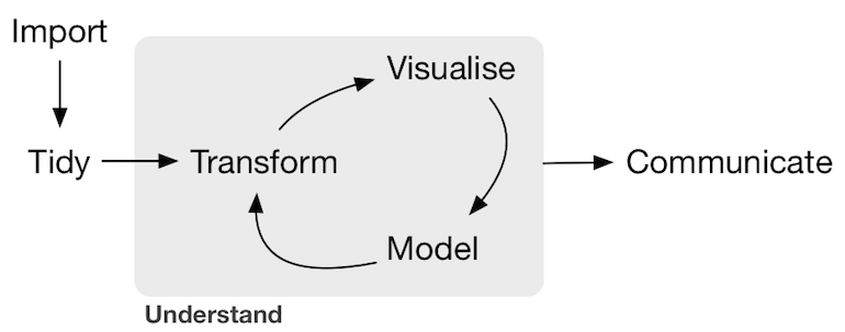 --- ## 1) Data First! Furthermore use data science tools <u>that a data scientist would use</u>. Example: [`tidyverse`](http://tidyverse.org/) <br> <center><img src="figure/hex.png" height="300px"/></center> --- ## 1) Data First! What does this buy us? * Students can do effective data storytelling * Context for asking scientific questions * Look at data that's rich, real, and realistic. Examples: Data packages such as [`nycflights13`](https://github.com/hadley/nycflights13) and [`fivethirtyeight`](https://cran.r-project.org/web/packages/fivethirtyeight/vignettes/fivethirtyeight.html) * Better motivate traditional statistical topics --- ## 2) Computers, Not Math! Cobb ([TAS 2015](https://arxiv.org/abs/1507.05346)): Two possible "computational engines" for statistics, in particular relating to sampling: * Mathematics: formulas, probability theory, large-sample approximations, central limit theorem -- * Computers: simulations, resampling methods --- ## 2) Computers, Not Math! We present students with a choice for our "engine": <br/> Either we use this... | Or we use this... :-------------------------:|:-------------------------: <img src="figure/formulas.png" alt="Drawing" style="width: 250px;"/> | <img src="figure/coding.jpg" alt="Drawing" style="width: 250px;"/> <br/> -- * Almost all are thrilled to do the latter -- * Leave "bread crumbs" for more advanced math/stats courses --- ## 2) Computers, Not Math! What does this buy us? * Emphasizes: stats is not math, rather stats uses math. * Simulations are more tactile * Reducing probability and march to CLT, this frees up space in syllabus. --- ## 3) Algorithms, Computation, & Coding * Both "Data First!" and "Computers, Not Math!" necessitate algorithmic thinking, computational logic, and some coding/programming. * Battle is more psychological than anything: + "This is not a class on programming!" + "Computers are stupid!" + "Learning to code is like learning a foreign language!" + "Early on don't code from scratch! Take something else that's similar and tweak it!" + Learning how to Google effectively --- ## 3) Algorithms, Computation, & Coding Why should we do this? * Data science and machine learning. * Where statistics is heading. Gelman [blog post](http://andrewgelman.com/2017/05/14/computer-programming-prerequisite-learning-statistics/). * If we don't, we are doing a disservice to students by shielding them from these computational ideas. * Bigger picture: Coding is becoming a basic skill like reading and writing. --- ## 4) Complete Reproducibility * Students learn best when they can take apart a toy (analysis) and then rebuild it (synthesis). * Crisis in Reproducibility * Ultimately the best textbook is one you've written yourself. + Everyone has different contexts, backgrounds, needs + Hard to find one-size-fits-all solutions * A new paradigm in textbooks? [Versions, not editions?](https://twitter.com/rudeboybert/status/820032345759592448) --- class: center, middle, inverse ## Let's Dive In! <a href="https://giphy.com/gifs/season-6-the-simpsons-6x1-l2Je1bFuOpkNpyqYM/"><img src="figure/homer.gif" style="width: 600px;"/></a> --- ## Baby's First Bookdown * ModernDive Light: Just Data Science Chapters of Bookdown * Download this ZIP file & extract the contents to a folder on your computer [`master.zip`](https://github.com/ismayc/moderndiver-lite/archive/master.zip) * Double click `moderndiver-lite.Rproj` to open in RStudio * Build -> Build Book - `install.packages('knitr', repos = c('http://rforge.net', 'http://cran.rstudio.org'), type = 'source')` --- <!-----------------------------------------------------------------------------> # Getting Started ## DataCamp DataCamp offers an interactive, browser based tool for learning R/Python. Their two flagship R courses, both of which are free: * [Intro to R](https://www.datacamp.com/courses/free-introduction-to-r) * [Intermediate R](https://www.datacamp.com/courses/intermediate-r-practice) courses --- ## DataCamp Outsource many essential but not fun to teach topics like * Idea of command-line vs point-and-click * Syntax: Variable names typed exactly, parentheses matching * Algorithmic Thinking: Linearity of code, object assignment * Computational Logic: boolean algebra, conditional statements, functions --- ## DataCamp Pros * Can assign "Intro to R" first day of class as "Homework 0" * Outsourcing allows you to free up class time * Students get immediate feedback on whether or not their code works + Often, the DataCamp error messages are much more useful than the ones R gives --- ## DataCamp Pros * With their [free academic license](https://www.datacamp.com/groups/education), you can + Form class "Groups" and assign/track progress of DataCamp courses + Have free access to ALL [their courses](https://www.datacamp.com/courses), including `ggplot2`, `dplyr`, `rmarkdown`, and RStudio IDE. + Create your own free DataCamp course covering content you want your students to learn using R --- ## DataCamp Cons * Some students will still have trouble; you can identify them however. * The topics in these two free courses may not align with your syllabus. You can assign at chapter level instead of course level though --- ## DataCamp Conclusion * Not a good tool for "quick retention," but for R concept introduction and subsequent repetition. + Students need to practice "speaking the language" just like with a foreign language. * [Feedback](https://docs.google.com/spreadsheets/d/1qUwt-v-xAQJ-1OTzMI2Q27McXG_3yXO5Qe9p-jz6BA8/edit) from students was positive. * Battle is more psychological than anything. DataCamp reinforces to students that + "Computers are stupid!" + "Learning to code is like learning a foreign language!" --- ## Chester's First Bookdown Project [Getting used to R, RStudio, and R Markdown](https://ismayc.github.io/rbasics-book/) - Designed to provide students with GIFs to follow along with and a description of all the components of RStudio and R Markdown --- class: inverse, center, middle ## Short break? --- ## Important R ideas for students to know ASAP Vector/variable - Type of vector (`int`, `num`, `chr`, `logical`, `date`) -- Data frame - Vectors of (potentially) different types - Each vector has the same number of rows --- class: center, middle # Welcome to the [tidyverse](https://blog.rstudio.org/2016/09/15/tidyverse-1-0-0/)! The `tidyverse` is a collection of R packages that share common philosophies and are designed to work together. <br><br> <a href="http://tidyverse.tidyverse.org/logo.png"><img src="figure/tidyverse.png" style="width: 200px;"/></a> --- # Chapter 3: Tidy Data? <img src="http://garrettgman.github.io/images/tidy-1.png" alt="Drawing" style="width: 750px;"/> 1. Each variable forms a column. 2. Each observation forms a row. 3. Each type of observational unit forms a table. The third point means we don't mix apples and oranges. --- ## What is Tidy Data? 1. Each observation forms a row. In other words, each row corresponds to a single instance of an <u>observational unit</u> 1. Each variable forms a column: + Some variables may be used to identify the <u>observational units</u>. + For organizational purposes, it's generally better to put these in the left-hand columns 1. Each type of observational unit forms a table. --- ## Differentiating between <u>neat</u> data and <u>tidy</u> data - Colloquially, they mean the same thing - But in our context, one is a subset of the other. <br> <u>Neat</u> data is - easy to look at, - organized nicely, and - in table form. -- <u>Tidy</u> data is neat but also abides by a set of three rules. --- class: center, middle <a href="figure/lebowski-abides-o.gif"><img src="http://stream1.gifsoup.com/view8/20150404/5192859/lebowski-abides-o.gif" style="width: 450px;"/></a> <img src="figure/tidy-1.png" alt="Drawing" style="width: 750px;"/> --- ## Is this tidy? ``` # A tibble: 12 × 4 year title clean_test budget_2013 <int> <chr> <chr> <int> 1 1995 Apollo 13 ok 99370665 2 2005 Brokeback Mountain notalk 16583160 3 2010 Diary of a Wimpy Kid ok 16023478 4 1984 Dune dubious 100864980 5 1984 Ghostbusters notalk 67243320 6 2003 How to Lose a Guy in 10 Days men 63304348 7 2011 Iris ok 5696299 8 2004 Sideways ok 20964279 9 2000 Songcatcher ok 2435235 10 2004 Team America: World Police men 24663858 11 2010 Tron Legacy notalk 213646368 12 2011 War Horse notalk 72498355 ``` --- name: demscore ## How about this? Is this tidy? ``` # A tibble: 12 × 13 country `1952` `1957` `1962` `1967` `1972` `1977` `1982` `1987` <chr> <int> <int> <int> <int> <int> <int> <int> <int> 1 Albania -9 -9 -9 -9 -9 -9 -9 -9 2 Argentina -9 -1 -1 -9 -9 -9 -8 8 3 Armenia -9 -7 -7 -7 -7 -7 -7 -7 4 Australia 10 10 10 10 10 10 10 10 5 Austria 10 10 10 10 10 10 10 10 6 Azerbaijan -9 -7 -7 -7 -7 -7 -7 -7 7 Belarus -9 -7 -7 -7 -7 -7 -7 -7 8 Belgium 10 10 10 10 10 10 10 10 9 Bhutan -10 -10 -10 -10 -10 -10 -10 -10 10 Bolivia -4 -3 -3 -4 -7 -7 8 9 11 Brazil 5 5 5 -9 -9 -4 -3 7 12 Bulgaria -7 -7 -7 -7 -7 -7 -7 -7 # ... with 4 more variables: `1992` <int>, `1997` <int>, `2002` <int>, # `2007` <int> ``` <small><small>[Why is tidy data important?](#whytidy) slide</small></small> --- ## Beginning steps Frequently the first thing to do when given a dataset is to - check that the data is <u>tidy</u>, - identify the observational unit, - specify the variables, and - give the types of variables you are presented with. This will help with - choosing the appropriate plot, - summarizing the data, and - understanding which inferences can be applied. --- class: center, middle # Chapter 4: Data Viz <a href="http://gitsense.github.io/images/wealth.gif"><img src="figure/wealth.gif" style="width: 770px;"/></a> Inspired by [Hans Rosling](https://www.youtube.com/watch?v=jbkSRLYSojo) --- <img src="slide_deck_files/figure-html/unnamed-chunk-4-1.png" style="display: block; margin: auto;" /> - What are the variables here? - What is the observational unit? - How are the variables mapped to aesthetics? --- class: center, middle ## Grammar of Graphics Wilkinson (2005) laid out the proposed <br> "Grammar of Graphics" <br> <a href="http://www.powells.com/book/the-grammar-of-graphics-9780387245447"><img src="figure/graphics.jpg" style="width: 200px;"></a> --- class: center, middle ## Grammar of Graphics in R Wickham implemented the grammar in R <br> in the `ggplot2` package <br> <a href="http://www.powells.com/book/ggplot2-elegant-graphics-for-data-analysis-9783319242750/68-428"><img src="figure/ggplot2.jpg" style="width: 200px;"></a> --- class: center, middle ## What is a statistical graphic? -- ## A `mapping` of <br> `data` variables -- ## to <br> `aes()`thetic attributes -- ## of <br> `geom_`etric objects. --- class: inverse, center, middle ## Back to basics --- ### Consider the following data in tidy format: ``` # A tibble: 4 × 4 A B C D <dbl> <dbl> <dbl> <chr> 1 1980 1 3 low 2 1990 2 2 low 3 2000 3 1 high 4 2010 4 2 high ``` <!-- Copy to chalkboard/whiteboard --> - Sketch the graphics below on paper, where the `x`-axis is variable `A` and the `y`-axis is variable `B` 1. <small>A scatter plot</small> 1. <small>A scatter plot where the `color` of the points corresponds to `D`</small> 1. <small>A scatter plot where the `size` of the points corresponds to `C`</small> 1. <small>A line graph</small> 1. <small>A line graph where the `color` of the line corresponds to `D` with points added that are all green of size 4.</small> --- ## Reproducing the plots in <small>`ggplot2`</small> ### 1. A scatterplot ```r library(ggplot2) ggplot(data = simple_ex, mapping = aes(x = A, y = B)) + geom_point() ``` -- 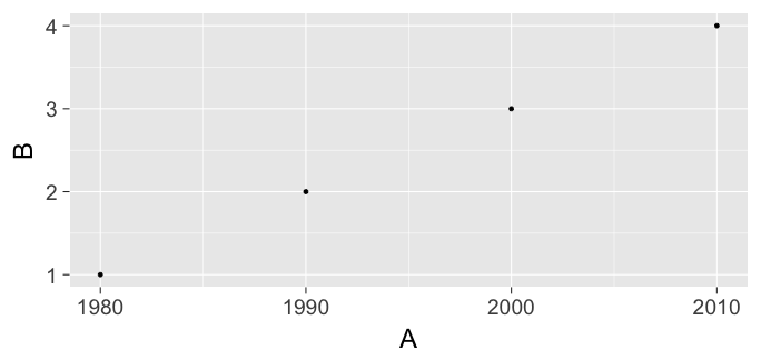<!-- --> --- ## Reproducing the plots in <small>`ggplot2`</small> ### 2. A scatter plot where the `color` of the points corresponds to `D` ```r library(ggplot2) ggplot(data = simple_ex, mapping = aes(x = A, y = B)) + geom_point(mapping = aes(color = D)) ``` -- 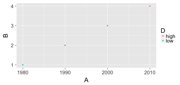<!-- --> --- ## Reproducing the plots in <small>`ggplot2`</small> ### 3. A scatter plot where the `size` of the points corresponds to `C` ```r library(ggplot2) ggplot(data = simple_ex, mapping = aes(x = A, y = B, size = C)) + geom_point() ``` -- 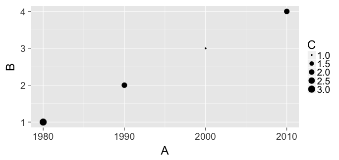<!-- --> --- ## Reproducing the plots in <small>`ggplot2`</small> ### 4. A line graph ```r library(ggplot2) ggplot(data = simple_ex, mapping = aes(x = A, y = B)) + geom_line() ``` -- 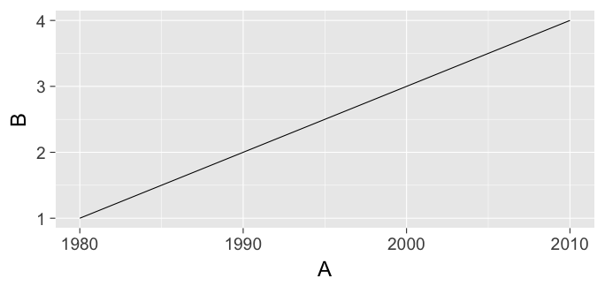<!-- --> --- ## Reproducing the plots in <small>`ggplot2`</small> ### 5. A line graph where the `color` of the line corresponds to `D` with points added that are all blue of size 4. ```r library(ggplot2) ggplot(data = simple_ex, mapping = aes(x = A, y = B)) + geom_line(mapping = aes(color = D)) + geom_point(color = "blue", size = 4) ``` -- 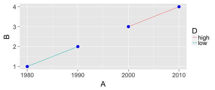<!-- --> --- name: whytidy ## Why is tidy data important? - Think about trying to plot democracy score across years in the simplest way possible with the data on the [Is this tidy? slide](#demscore). -- - It would be much easier if the data looked like what follows instead so we could put - `year` on the `x`-axis and - `dem_score` on the `y`-axis. --- ## Tidy is good ``` # A tibble: 13 × 3 country year dem_score <chr> <dbl> <int> 1 Argentina 1962 -1 2 Armenia 1997 -6 3 Denmark 1962 10 4 Ethiopia 2007 1 5 Finland 2007 10 6 Ireland 1992 10 7 Libya 1957 -7 8 Libya 1982 -7 9 Mexico 1977 -3 10 Mexico 1982 -3 11 Spain 1962 -7 12 Switzerland 1982 10 13 Ukraine 1997 7 ``` --- ## Let's plot it - Plot the line graph for 4 countries using `ggplot` ```r dem_score4 <- dem_score_tidy %>% filter(country %in% c("Australia", "Pakistan", "Portugal", "Uruguay")) ggplot(data = dem_score4, mapping = aes(x = year, y = dem_score)) + geom_line(mapping = aes(color = country)) ``` 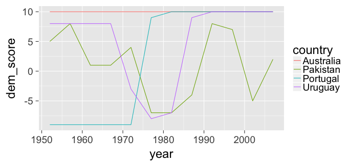<!-- --> --- # The Five-Named Graphs ## The 5NG of data viz - Scatterplot: `geom_point()` - Line graph: `geom_line()` -- - Histogram: `geom_histogram()` - Boxplot: `geom_boxplot()` - Bar graph: `geom_bar()` --- class: center, middle ## More examples --- ## Histogram ```r library(nycflights13) ggplot(data = weather, mapping = aes(x = humid)) + geom_histogram(bins = 20, color = "black", fill = "darkorange") ``` 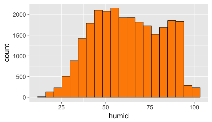<!-- --> --- ## Boxplot (broken) ```r library(nycflights13) ggplot(data = weather, mapping = aes(x = month, y = humid)) + geom_boxplot() ``` <!-- --> --- ## Boxplot (fixed) ```r library(nycflights13) ggplot(data = weather, mapping = aes(x = factor(month), y = humid)) + geom_boxplot() ``` <!-- --> --- ## Bar graph ```r library(fivethirtyeight) ggplot(data = bechdel, mapping = aes(x = clean_test)) + geom_bar() ``` <!-- --> --- ## How about over time? - Hop into `dplyr` ```r library(dplyr) year_bins <- c("'70-'74", "'75-'79", "'80-'84", "'85-'89", "'90-'94", "'95-'99", "'00-'04", "'05-'09", "'10-'13") bechdel <- bechdel %>% mutate(five_year = cut(year, breaks = seq(1969, 2014, 5), labels = year_bins)) %>% mutate(clean_test = factor(clean_test, levels = c("nowomen", "notalk", "men", "dubious", "ok"))) ``` --- ## How about over time? (Stacked) ```r library(fivethirtyeight) library(ggplot2) ggplot(data = bechdel, mapping = aes(x = five_year, fill = clean_test)) + geom_bar() ``` <!-- --> --- ## How about over time? (Side-by-side) ```r library(fivethirtyeight) library(ggplot2) ggplot(data = bechdel, mapping = aes(x = five_year, fill = clean_test)) + geom_bar(position = "dodge") ``` 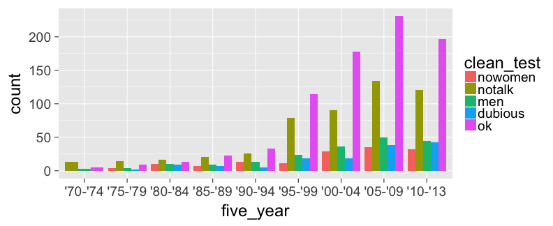<!-- --> --- ## How about over time? (Stacked proportional) ```r library(fivethirtyeight) library(ggplot2) ggplot(data = bechdel, mapping = aes(x = five_year, fill = clean_test)) + geom_bar(position = "fill", color = "black") ``` 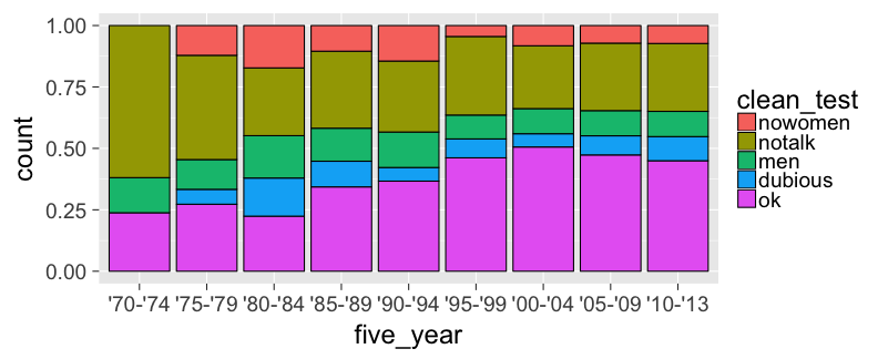<!-- --> --- class: center, middle ## `ggplot2` is for beginners and for data science professionals! <a href="https://fivethirtyeight.com/features/the-dollar-and-cents-case-against-hollywoods-exclusion-of-women/"><img src="figure/bechdel.png" width=500></a> --- ## Practice Produce appropriate 5NG with R package & data set in [ ], e.g., [`nycflights13` `\(\rightarrow\)` `weather`] <!-- Try to look through the help documentation/Google to improve your plots --> 1. Does `age` predict `recline_rude`? <br> [`fivethirtyeight` `\(\rightarrow\)` `na.omit(flying)`] 2. Distribution of `age` by `sex` <br> [`okcupiddata` `\(\rightarrow\)` `profiles`] 3. Does `budget` predict `rating`? <br> [`ggplot2movies` `\(\rightarrow\)` `movies`] 4. Distribution of log base 10 scale of `budget_2013` <br> [`fivethirtyeight` `\(\rightarrow\)` `bechdel`] --- ### HINTS 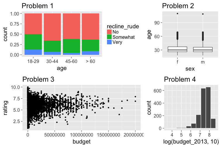<!-- --> --- class: inverse, center, middle # DEMO in RStudio --- class: center, middle ### Determining the appropriate plot <a href="https://coggle.it/diagram/V_G2gzukTDoQ-aZt"><img src="figure/viz_mindmap.png" style="width: 400px;"/></a> --- class: center, middle # Chapter 5: Data Wrangling --- ### `gapminder` data frame in the `gapminder` package ```r library(gapminder) gapminder ``` ``` # A tibble: 1,704 × 6 country continent year lifeExp pop gdpPercap <fctr> <fctr> <int> <dbl> <int> <dbl> 1 Afghanistan Asia 1952 28.801 8425333 779.4453 2 Afghanistan Asia 1957 30.332 9240934 820.8530 3 Afghanistan Asia 1962 31.997 10267083 853.1007 4 Afghanistan Asia 1967 34.020 11537966 836.1971 5 Afghanistan Asia 1972 36.088 13079460 739.9811 6 Afghanistan Asia 1977 38.438 14880372 786.1134 7 Afghanistan Asia 1982 39.854 12881816 978.0114 8 Afghanistan Asia 1987 40.822 13867957 852.3959 9 Afghanistan Asia 1992 41.674 16317921 649.3414 10 Afghanistan Asia 1997 41.763 22227415 635.3414 # ... with 1,694 more rows ``` --- ## Base R versus the `tidyverse` Say we wanted mean life expectancy across all years for Asia -- ```r # Base R asia <- gapminder[gapminder$continent == "Asia", ] mean(asia$lifeExp) ``` ``` [1] 60.0649 ``` -- ```r library(dplyr) gapminder %>% filter(continent == "Asia") %>% summarize(mean_exp = mean(lifeExp)) ``` ``` # A tibble: 1 × 1 mean_exp <dbl> 1 60.0649 ``` --- ## The pipe `%>%` <img src="figure/pipe.png" width="245" />    <!-- --> -- - A way to chain together commands -- - It is *essentially* the `dplyr` equivalent to the <br> `+` in `ggplot2` --- ## The 5NG of data viz -- ### `geom_point()`<br> `geom_line()` <br> `geom_histogram()`<br> `geom_boxplot()`<br> `geom_bar()` --- # The Five Main Verbs (5MV) of data wrangling ### `filter()` <br> `summarize()` <br> `group_by()` <br> `mutate()` <br> `arrange()` --- ## `filter()` - Select a subset of the rows of a data frame. - The arguments are the "filters" that you'd like to apply. -- ```r library(gapminder); library(dplyr) gap_2007 <- gapminder %>% filter(year == 2007) head(gap_2007) ``` ``` # A tibble: 6 × 6 country continent year lifeExp pop gdpPercap <fctr> <fctr> <int> <dbl> <int> <dbl> 1 Afghanistan Asia 2007 43.828 31889923 974.5803 2 Albania Europe 2007 76.423 3600523 5937.0295 3 Algeria Africa 2007 72.301 33333216 6223.3675 4 Angola Africa 2007 42.731 12420476 4797.2313 5 Argentina Americas 2007 75.320 40301927 12779.3796 6 Australia Oceania 2007 81.235 20434176 34435.3674 ``` - Use `==` to compare a variable to a value --- ## Logical operators - Use `|` to check for any in multiple filters being true: -- ```r gapminder %>% filter(year == 2002 | continent == "Europe") ``` -- ``` # A tibble: 472 × 6 country continent year lifeExp pop gdpPercap <fctr> <fctr> <int> <dbl> <int> <dbl> 1 Afghanistan Asia 2002 42.129 25268405 726.7341 2 Albania Europe 1952 55.230 1282697 1601.0561 3 Albania Europe 1957 59.280 1476505 1942.2842 4 Albania Europe 1962 64.820 1728137 2312.8890 5 Albania Europe 1967 66.220 1984060 2760.1969 6 Albania Europe 1972 67.690 2263554 3313.4222 7 Albania Europe 1977 68.930 2509048 3533.0039 8 Albania Europe 1982 70.420 2780097 3630.8807 9 Albania Europe 1987 72.000 3075321 3738.9327 10 Albania Europe 1992 71.581 3326498 2497.4379 # ... with 462 more rows ``` --- ## Logical operators - Use `&` or `,` to check for all of multiple filters being true: -- ```r gapminder %>% filter(year == 2002, continent == "Europe") ``` ``` # A tibble: 30 × 6 country continent year lifeExp pop gdpPercap <fctr> <fctr> <int> <dbl> <int> <dbl> 1 Albania Europe 2002 75.651 3508512 4604.212 2 Austria Europe 2002 78.980 8148312 32417.608 3 Belgium Europe 2002 78.320 10311970 30485.884 4 Bosnia and Herzegovina Europe 2002 74.090 4165416 6018.975 5 Bulgaria Europe 2002 72.140 7661799 7696.778 6 Croatia Europe 2002 74.876 4481020 11628.389 7 Czech Republic Europe 2002 75.510 10256295 17596.210 8 Denmark Europe 2002 77.180 5374693 32166.500 9 Finland Europe 2002 78.370 5193039 28204.591 10 France Europe 2002 79.590 59925035 28926.032 # ... with 20 more rows ``` --- ## Logical operators - Use `%in%` to check for any being true <br> (shortcut to using `|` repeatedly with `==`) -- ```r gapminder %>% filter(country %in% c("Argentina", "Belgium", "Mexico"), year %in% c(1987, 1992)) ``` -- ``` # A tibble: 6 × 6 country continent year lifeExp pop gdpPercap <fctr> <fctr> <int> <dbl> <int> <dbl> 1 Argentina Americas 1987 70.774 31620918 9139.671 2 Argentina Americas 1992 71.868 33958947 9308.419 3 Belgium Europe 1987 75.350 9870200 22525.563 4 Belgium Europe 1992 76.460 10045622 25575.571 5 Mexico Americas 1987 69.498 80122492 8688.156 6 Mexico Americas 1992 71.455 88111030 9472.384 ``` --- ## `summarize()` - Any numerical summary that you want to apply to a column of a data frame is specified within `summarize()`. ```r max_exp_1997 <- gapminder %>% filter(year == 1997) %>% summarize(max_exp = max(lifeExp)) max_exp_1997 ``` -- ``` # A tibble: 1 × 1 max_exp <dbl> 1 80.69 ``` --- ### Combining `summarize()` with `group_by()` When you'd like to determine a numerical summary for all levels of a different categorical variable ```r max_exp_1997_by_cont <- gapminder %>% filter(year == 1997) %>% group_by(continent) %>% summarize(max_exp = max(lifeExp), sd_exp = sd(lifeExp)) max_exp_1997_by_cont ``` -- ``` # A tibble: 5 × 3 continent max_exp sd_exp <fctr> <dbl> <dbl> 1 Africa 74.772 9.1033866 2 Americas 78.610 4.8875839 3 Asia 80.690 8.0911706 4 Europe 79.390 3.1046766 5 Oceania 78.830 0.9050967 ``` --- ## `ggplot2` revisited For aggregated data, use `geom_col`. (A dynamite plot is also shown.) ```r ggplot(data = max_exp_1997_by_cont, mapping = aes(x = continent, y = max_exp)) + geom_col(fill = "red") + geom_errorbar(mapping = aes(ymin = max_exp - sd_exp, ymax = max_exp + sd_exp), color = "blue", width = 0.2) ``` <!-- --> --- ## The 5MV - `filter()` - `summarize()` - `group_by()` -- - `mutate()` -- - `arrange()` --- ## `mutate()` - Allows you to 1. <font color="blue">create a new variable with a specific value</font> OR 2. create a new variable based on other variables OR 3. change the contents of an existing variable -- ```r gap_plus <- gapminder %>% mutate(just_one = 1) head(gap_plus) ``` ``` # A tibble: 6 × 7 country continent year lifeExp pop gdpPercap just_one <fctr> <fctr> <int> <dbl> <int> <dbl> <dbl> 1 Afghanistan Asia 1952 28.801 8425333 779.4453 1 2 Afghanistan Asia 1957 30.332 9240934 820.8530 1 3 Afghanistan Asia 1962 31.997 10267083 853.1007 1 4 Afghanistan Asia 1967 34.020 11537966 836.1971 1 5 Afghanistan Asia 1972 36.088 13079460 739.9811 1 6 Afghanistan Asia 1977 38.438 14880372 786.1134 1 ``` --- ## `mutate()` - Allows you to 1. create a new variable with a specific value OR 2. <font color="blue">create a new variable based on other variables</font> OR 3. change the contents of an existing variable -- ```r gap_w_gdp <- gapminder %>% mutate(gdp = pop * gdpPercap) head(gap_w_gdp) ``` ``` # A tibble: 6 × 7 country continent year lifeExp pop gdpPercap gdp <fctr> <fctr> <int> <dbl> <int> <dbl> <dbl> 1 Afghanistan Asia 1952 28.801 8425333 779.4453 6567086330 2 Afghanistan Asia 1957 30.332 9240934 820.8530 7585448670 3 Afghanistan Asia 1962 31.997 10267083 853.1007 8758855797 4 Afghanistan Asia 1967 34.020 11537966 836.1971 9648014150 5 Afghanistan Asia 1972 36.088 13079460 739.9811 9678553274 6 Afghanistan Asia 1977 38.438 14880372 786.1134 11697659231 ``` --- ## `mutate()` - Allows you to 1. create a new variable with a specific value OR 2. create a new variable based on other variables OR 3. <font color="blue">change the contents of an existing variable</font> -- ```r gap_weird <- gapminder %>% mutate(pop = pop + 1000) head(gap_weird) ``` ``` # A tibble: 6 × 6 country continent year lifeExp pop gdpPercap <fctr> <fctr> <int> <dbl> <dbl> <dbl> 1 Afghanistan Asia 1952 28.801 8426333 779.4453 2 Afghanistan Asia 1957 30.332 9241934 820.8530 3 Afghanistan Asia 1962 31.997 10268083 853.1007 4 Afghanistan Asia 1967 34.020 11538966 836.1971 5 Afghanistan Asia 1972 36.088 13080460 739.9811 6 Afghanistan Asia 1977 38.438 14881372 786.1134 ``` --- ## `arrange()` - Reorders the rows in a data frame based on the values of one or more variables -- ```r gapminder %>% arrange(year, country) ``` ``` # A tibble: 1,704 × 6 country continent year lifeExp pop gdpPercap <fctr> <fctr> <int> <dbl> <int> <dbl> 1 Afghanistan Asia 1952 28.801 8425333 779.4453 2 Albania Europe 1952 55.230 1282697 1601.0561 3 Algeria Africa 1952 43.077 9279525 2449.0082 4 Angola Africa 1952 30.015 4232095 3520.6103 5 Argentina Americas 1952 62.485 17876956 5911.3151 6 Australia Oceania 1952 69.120 8691212 10039.5956 7 Austria Europe 1952 66.800 6927772 6137.0765 8 Bahrain Asia 1952 50.939 120447 9867.0848 9 Bangladesh Asia 1952 37.484 46886859 684.2442 10 Belgium Europe 1952 68.000 8730405 8343.1051 # ... with 1,694 more rows ``` --- ## `arrange()` - Can also put into descending order -- ```r gapminder %>% filter(year > 2000) %>% arrange(desc(lifeExp)) %>% head(10) ``` ``` # A tibble: 10 × 6 country continent year lifeExp pop gdpPercap <fctr> <fctr> <int> <dbl> <int> <dbl> 1 Japan Asia 2007 82.603 127467972 31656.07 2 Hong Kong, China Asia 2007 82.208 6980412 39724.98 3 Japan Asia 2002 82.000 127065841 28604.59 4 Iceland Europe 2007 81.757 301931 36180.79 5 Switzerland Europe 2007 81.701 7554661 37506.42 6 Hong Kong, China Asia 2002 81.495 6762476 30209.02 7 Australia Oceania 2007 81.235 20434176 34435.37 8 Spain Europe 2007 80.941 40448191 28821.06 9 Sweden Europe 2007 80.884 9031088 33859.75 10 Israel Asia 2007 80.745 6426679 25523.28 ``` --- ## Don't mix up `arrange` and `group_by` - `group_by` is used (mostly) with `summarize` to calculate summaries over groups - `arrange` is used for sorting --- ## Don't mix up `arrange` and `group_by` This doesn't really do anything useful ```r gapminder %>% group_by(year) ``` ``` Source: local data frame [1,704 x 6] Groups: year [12] country continent year lifeExp pop gdpPercap <fctr> <fctr> <int> <dbl> <int> <dbl> 1 Afghanistan Asia 1952 28.801 8425333 779.4453 2 Afghanistan Asia 1957 30.332 9240934 820.8530 3 Afghanistan Asia 1962 31.997 10267083 853.1007 4 Afghanistan Asia 1967 34.020 11537966 836.1971 5 Afghanistan Asia 1972 36.088 13079460 739.9811 6 Afghanistan Asia 1977 38.438 14880372 786.1134 7 Afghanistan Asia 1982 39.854 12881816 978.0114 8 Afghanistan Asia 1987 40.822 13867957 852.3959 9 Afghanistan Asia 1992 41.674 16317921 649.3414 10 Afghanistan Asia 1997 41.763 22227415 635.3414 # ... with 1,694 more rows ``` --- ## Don't mix up `arrange` and `group_by` But this does ```r gapminder %>% arrange(year) ``` ``` # A tibble: 1,704 × 6 country continent year lifeExp pop gdpPercap <fctr> <fctr> <int> <dbl> <int> <dbl> 1 Afghanistan Asia 1952 28.801 8425333 779.4453 2 Albania Europe 1952 55.230 1282697 1601.0561 3 Algeria Africa 1952 43.077 9279525 2449.0082 4 Angola Africa 1952 30.015 4232095 3520.6103 5 Argentina Americas 1952 62.485 17876956 5911.3151 6 Australia Oceania 1952 69.120 8691212 10039.5956 7 Austria Europe 1952 66.800 6927772 6137.0765 8 Bahrain Asia 1952 50.939 120447 9867.0848 9 Bangladesh Asia 1952 37.484 46886859 684.2442 10 Belgium Europe 1952 68.000 8730405 8343.1051 # ... with 1,694 more rows ``` --- ## Changing of observation unit True or False > Each of `filter`, `mutate`, and `arrange` change the observational unit. -- True or False > `group_by() %>% summarize()` changes the observational unit. <!-- Draw diagram for average monthly temp aggregated like on rstudio::conf slides --> --- class: center ## What is meant by "joining data frames" and <br> why is it useful? -- <img src="https://ismayc.github.io/moderndiver-book/images/join-inner.png" style="display: block; margin: auto;" /> --- ### Does cost of living in a state relate to whether police officers live in the cities they patrol? What about state political ideology? ```r library(fivethirtyeight) library(readr) ideology <- read_csv("https://ismayc.github.io/Effective-Data-Storytelling-using-the-tidyverse/datasets/ideology.csv") police_join <- inner_join(x = police_locals, y = ideology, by = "city") rmarkdown::paged_table(police_join) ``` <div data-pagedtable="false"> <script data-pagedtable-source type="application/json"> {"columns":[{"label":["city"],"name":[1],"type":["chr"],"align":["left"]},{"label":["force_size"],"name":[2],"type":["int"],"align":["right"]},{"label":["all"],"name":[3],"type":["dbl"],"align":["right"]},{"label":["white"],"name":[4],"type":["dbl"],"align":["right"]},{"label":["non_white"],"name":[5],"type":["dbl"],"align":["right"]},{"label":["black"],"name":[6],"type":["dbl"],"align":["right"]},{"label":["hispanic"],"name":[7],"type":["dbl"],"align":["right"]},{"label":["asian"],"name":[8],"type":["dbl"],"align":["right"]},{"label":["state"],"name":[9],"type":["chr"],"align":["left"]},{"label":["state_ideology"],"name":[10],"type":["chr"],"align":["left"]}],"data":[{"1":"New York","2":"32300","3":"0.61795666","4":"0.44638656","5":"0.76441894","6":"0.7708914","7":"0.76286073","8":"0.7492355","9":"New York","10":"Liberal"},{"1":"Chicago","2":"12120","3":"0.87500000","4":"0.87196262","5":"0.87740030","6":"0.8974057","7":"0.83982684","8":"0.9666667","9":"Illinois","10":"Liberal"},{"1":"Los Angeles","2":"10100","3":"0.22821782","4":"0.15277778","5":"0.26384840","6":"0.3873874","7":"0.21767956","8":"0.3052632","9":"California","10":"Liberal"},{"1":"Washington","2":"9340","3":"0.11563169","4":"0.05677419","5":"0.15736505","6":"0.1701891","7":"0.08988764","8":"0.2307692","9":"District of Columbia","10":"Liberal"},{"1":"Houston","2":"7700","3":"0.29220779","4":"0.17373461","5":"0.39925834","6":"0.3663793","7":"0.45714286","8":"0.4081633","9":"Texas","10":"Conservative"},{"1":"Philadelphia","2":"6045","3":"0.83540116","4":"0.77689873","5":"0.89948007","6":"0.9246575","7":"0.81739130","8":"NA","9":"Pennsylvania","10":"Conservative"},{"1":"Phoenix","2":"4475","3":"0.31173184","4":"0.27080182","5":"0.42735043","6":"0.5217391","7":"0.42771084","8":"NA","9":"Arizona","10":"Conservative"},{"1":"San Diego","2":"4460","3":"0.36210762","4":"0.37298387","5":"0.34848485","6":"0.5384615","7":"0.29779412","8":"0.5156250","9":"California","10":"Liberal"},{"1":"Dallas","2":"3605","3":"0.19140083","4":"0.17150396","5":"0.21345029","6":"0.2146341","7":"0.25688073","8":"NA","9":"Texas","10":"Conservative"},{"1":"Detroit","2":"3265","3":"0.37059724","4":"0.08196721","5":"0.54278729","6":"0.5680000","7":"0.33333333","8":"NA","9":"Michigan","10":"Conservative"},{"1":"San Francisco","2":"3020","3":"0.31622517","4":"0.25949367","5":"0.37847222","6":"0.1860465","7":"0.25333333","8":"0.4861111","9":"California","10":"Liberal"},{"1":"San Antonio","2":"2955","3":"0.62436548","4":"0.44387755","5":"0.71392405","6":"0.5744681","7":"0.73913043","8":"NA","9":"Texas","10":"Conservative"},{"1":"Atlanta","2":"2950","3":"0.13728814","4":"0.18627451","5":"0.11139896","6":"0.1019830","7":"NA","8":"NA","9":"Georgia","10":"Conservative"},{"1":"Las Vegas","2":"2830","3":"0.37455830","4":"0.40000000","5":"0.30769231","6":"0.3877551","7":"0.26785714","8":"NA","9":"Nevada","10":"Liberal"},{"1":"Baltimore","2":"2800","3":"0.25714286","4":"0.13281250","5":"0.36184211","6":"0.3914591","7":"NA","8":"NA","9":"Maryland","10":"Liberal"},{"1":"Boston","2":"2560","3":"0.47656250","4":"0.44155844","5":"0.58267716","6":"0.6865672","7":"0.75000000","8":"NA","9":"Massachusetts","10":"Liberal"},{"1":"Jacksonville, Fla.","2":"2335","3":"0.80942184","4":"0.71378092","5":"0.95652174","6":"1.0000000","7":"0.88888889","8":"1.0000000","9":"Florida","10":"Conservative"},{"1":"El Paso, Texas","2":"2260","3":"0.85176991","4":"0.82644628","5":"0.86102719","6":"NA","7":"0.86102719","8":"NA","9":"Texas","10":"Conservative"},{"1":"Columbus, Ohio","2":"2245","3":"0.40534521","4":"0.37978142","5":"0.51807229","6":"0.5714286","7":"NA","8":"NA","9":"Ohio","10":"Conservative"},{"1":"Cleveland","2":"2045","3":"0.55745721","4":"0.49812734","5":"0.66901409","6":"0.5959596","7":"0.94117647","8":"NA","9":"Ohio","10":"Conservative"},{"1":"Tucson, Ariz.","2":"2020","3":"0.39851485","4":"0.41666667","5":"0.37500000","6":"NA","7":"0.33333333","8":"NA","9":"Arizona","10":"Conservative"},{"1":"Newark, N.J.","2":"2005","3":"0.27930175","4":"0.20796460","5":"0.37142857","6":"0.5194805","7":"0.26041667","8":"NA","9":"New Jersey","10":"Liberal"},{"1":"Austin, Texas","2":"1985","3":"0.29471033","4":"0.19469027","5":"0.42690058","6":"0.2500000","7":"0.45384615","8":"NA","9":"Texas","10":"Conservative"},{"1":"Memphis, Tenn.","2":"1970","3":"0.46446700","4":"0.33913044","5":"0.64024390","6":"0.6688742","7":"NA","8":"NA","9":"Tennessee","10":"Conservative"},{"1":"Milwaukee","2":"1960","3":"0.72193878","4":"0.69288390","5":"0.78400000","6":"0.9310345","7":"0.73333333","8":"NA","9":"Wisconsin","10":"Conservative"},{"1":"San Jose, Calif.","2":"1875","3":"0.46666667","4":"0.47234043","5":"0.45714286","6":"NA","7":"0.40697674","8":"0.4400000","9":"California","10":"Liberal"},{"1":"Miami","2":"1860","3":"0.07258064","4":"0.03061224","5":"0.08759124","6":"0.0000000","7":"0.11675127","8":"NA","9":"Florida","10":"Conservative"},{"1":"Denver","2":"1820","3":"0.28296703","4":"0.14932127","5":"0.48951049","6":"0.5806452","7":"0.39175258","8":"NA","9":"Colorado","10":"Liberal"},{"1":"Sacramento, Calif.","2":"1820","3":"0.07967033","4":"0.06338028","5":"0.13750000","6":"0.3200000","7":"0.00000000","8":"NA","9":"California","10":"Liberal"},{"1":"Charlotte, N.C.","2":"1780","3":"0.36235955","4":"0.29454546","5":"0.59259259","6":"0.8333333","7":"0.32142857","8":"NA","9":"North Carolina","10":"Conservative"},{"1":"Tampa, Fla.","2":"1715","3":"0.17784257","4":"0.13191489","5":"0.27777778","6":"0.2765957","7":"0.32692308","8":"NA","9":"Florida","10":"Conservative"},{"1":"Indianapolis","2":"1620","3":"0.64814815","4":"0.71042471","5":"0.40000000","6":"0.3833333","7":"NA","8":"NA","9":"Indiana","10":"Conservative"},{"1":"Santa Ana, Calif.","2":"1590","3":"0.09433962","4":"0.05882353","5":"0.12087912","6":"NA","7":"0.14864865","8":"0.0000000","9":"California","10":"Liberal"},{"1":"New Orleans","2":"1560","3":"0.50000000","4":"0.32407407","5":"0.59313726","6":"0.6237113","7":"NA","8":"NA","9":"Louisiana","10":"Conservative"},{"1":"Oakland, Calif.","2":"1530","3":"0.09477124","4":"0.02666667","5":"0.16025641","6":"0.0625000","7":"0.10810811","8":"0.2812500","9":"California","10":"Liberal"},{"1":"Orlando, Fla.","2":"1530","3":"0.11764706","4":"0.09000000","5":"0.16981132","6":"NA","7":"0.11111111","8":"NA","9":"Florida","10":"Conservative"},{"1":"Oklahoma City, Okla.","2":"1500","3":"0.59666667","4":"0.54732510","5":"0.80701754","6":"0.6296296","7":"NA","8":"NA","9":"Oklahoma","10":"Conservative"},{"1":"Seattle","2":"1445","3":"0.11764706","4":"0.11557789","5":"0.12222222","6":"0.1875000","7":"0.00000000","8":"NA","9":"Washington","10":"Liberal"},{"1":"Kansas City, Mo.","2":"1440","3":"0.77777778","4":"0.76800000","5":"0.84210526","6":"1.0000000","7":"NA","8":"NA","9":"Missouri","10":"Conservative"},{"1":"Nashville, Tenn.","2":"1440","3":"0.61805556","4":"0.43715847","5":"0.93333333","6":"0.9473684","7":"NA","8":"NA","9":"Tennessee","10":"Conservative"},{"1":"Laredo, Texas","2":"1435","3":"0.93728223","4":"0.96296296","5":"0.93133047","6":"NA","7":"0.93133047","8":"NA","9":"Texas","10":"Conservative"},{"1":"Fort Worth, Texas","2":"1430","3":"0.42657343","4":"0.30674847","5":"0.58536585","6":"0.6379310","7":"0.55932203","8":"NA","9":"Texas","10":"Conservative"},{"1":"Louisville, Ky.","2":"1430","3":"0.64685315","4":"0.62083333","5":"0.78260870","6":"0.7727273","7":"NA","8":"NA","9":"Kentucky","10":"Conservative"},{"1":"Norfolk, Va.","2":"1425","3":"0.21754386","4":"0.26708075","5":"0.15322581","6":"0.1067961","7":"NA","8":"NA","9":"Virginia","10":"Liberal"},{"1":"Arlington, Va.","2":"1360","3":"0.20220588","4":"0.22222222","5":"0.17968750","6":"0.1600000","7":"NA","8":"NA","9":"Virginia","10":"Liberal"},{"1":"Pittsburgh","2":"1350","3":"0.65925926","4":"0.67965368","5":"0.53846154","6":"0.5333333","7":"NA","8":"NA","9":"Pennsylvania","10":"Conservative"},{"1":"Albuquerque, N.M.","2":"1340","3":"0.61567164","4":"0.62962963","5":"0.60150376","6":"NA","7":"0.56637168","8":"NA","9":"New Mexico","10":"Liberal"},{"1":"Jersey City, N.J.","2":"1170","3":"0.25213675","4":"0.20645161","5":"0.34177215","6":"0.3030303","7":"0.32558139","8":"NA","9":"New Jersey","10":"Liberal"},{"1":"Raleigh, N.C.","2":"1150","3":"0.26956522","4":"0.20634921","5":"0.56097561","6":"NA","7":"NA","8":"NA","9":"North Carolina","10":"Conservative"},{"1":"Rochester, N.Y.","2":"1150","3":"0.10000000","4":"0.04093567","5":"0.27118644","6":"0.1951220","7":"NA","8":"NA","9":"New York","10":"Liberal"},{"1":"Cincinnati","2":"1145","3":"0.22707424","4":"0.14772727","5":"0.49056604","6":"0.6486486","7":"NA","8":"NA","9":"Ohio","10":"Conservative"},{"1":"Long Beach, Calif.","2":"1115","3":"0.29147982","4":"0.27722772","5":"0.30327869","6":"NA","7":"0.31250000","8":"0.0000000","9":"California","10":"Liberal"},{"1":"Birmingham, Ala.","2":"1110","3":"0.22522523","4":"0.08602150","5":"0.32558139","6":"0.3281250","7":"NA","8":"NA","9":"Alabama","10":"Conservative"},{"1":"Wichita, Kan.","2":"1075","3":"0.60000000","4":"0.51176471","5":"0.93333333","6":"NA","7":"0.89655172","8":"NA","9":"Kansas","10":"Conservative"},{"1":"Virginia Beach, Va.","2":"1070","3":"0.78971963","4":"0.75625000","5":"0.88888889","6":"0.7272727","7":"1.00000000","8":"NA","9":"Virginia","10":"Liberal"},{"1":"Fresno, Calif.","2":"1040","3":"0.51442308","4":"0.50961539","5":"0.51923077","6":"0.6818182","7":"0.46031746","8":"NA","9":"California","10":"Liberal"},{"1":"Buffalo, N.Y.","2":"1010","3":"0.33663366","4":"0.29239766","5":"0.58064516","6":"NA","7":"0.52380952","8":"NA","9":"New York","10":"Liberal"},{"1":"Minneapolis","2":"1000","3":"0.10000000","4":"0.05263158","5":"0.37931034","6":"NA","7":"NA","8":"NA","9":"Minnesota","10":"Liberal"},{"1":"Portland, Ore.","2":"1000","3":"0.21000000","4":"0.18644068","5":"0.39130435","6":"NA","7":"NA","8":"NA","9":"Oregon","10":"Liberal"},{"1":"Reno, Nev.","2":"1000","3":"0.34000000","4":"0.32386364","5":"0.45833333","6":"NA","7":"NA","8":"NA","9":"Nevada","10":"Liberal"},{"1":"Richmond, Va.","2":"1000","3":"0.11000000","4":"0.10169491","5":"0.12195122","6":"0.2083333","7":"NA","8":"NA","9":"Virginia","10":"Liberal"},{"1":"Baton Rouge, La.","2":"980","3":"0.21428571","4":"0.14406780","5":"0.32051282","6":"0.3424658","7":"NA","8":"NA","9":"Louisiana","10":"Conservative"},{"1":"Jackson, Miss.","2":"960","3":"0.39062500","4":"0.08219178","5":"0.57983193","6":"0.5798319","7":"NA","8":"NA","9":"Mississippi","10":"Conservative"},{"1":"Riverside, Calif.","2":"955","3":"0.21989529","4":"0.35000000","5":"0.07692308","6":"0.0000000","7":"0.14285714","8":"NA","9":"California","10":"Liberal"},{"1":"Fort Lauderdale, Fla.","2":"950","3":"0.16842105","4":"0.22018349","5":"0.09876543","6":"0.1025641","7":"0.11428571","8":"NA","9":"Florida","10":"Conservative"},{"1":"St. Louis","2":"950","3":"0.58947368","4":"0.53846154","5":"0.67123288","6":"0.6825397","7":"NA","8":"NA","9":"Missouri","10":"Conservative"},{"1":"Brownsville, Texas","2":"925","3":"0.51351351","4":"0.50000000","5":"0.51412429","6":"NA","7":"0.52023121","8":"NA","9":"Texas","10":"Conservative"},{"1":"Albany, N.Y.","2":"890","3":"0.18539326","4":"0.16025641","5":"0.36363636","6":"NA","7":"NA","8":"NA","9":"New York","10":"Liberal"},{"1":"Colorado Springs, Colo.","2":"860","3":"0.60465116","4":"0.55303030","5":"0.77500000","6":"NA","7":"0.91304348","8":"NA","9":"Colorado","10":"Liberal"},{"1":"Savannah, Ga.","2":"860","3":"0.21511628","4":"0.07692308","5":"0.29906542","6":"0.1707317","7":"0.75000000","8":"NA","9":"Georgia","10":"Conservative"},{"1":"Winston-Salem, N.C.","2":"860","3":"0.57558140","4":"0.42477876","5":"0.86440678","6":"0.8695652","7":"NA","8":"NA","9":"North Carolina","10":"Conservative"},{"1":"Toledo, Ohio","2":"805","3":"0.56521739","4":"0.53076923","5":"0.70967742","6":"0.7500000","7":"NA","8":"NA","9":"Ohio","10":"Conservative"},{"1":"Madison, Wis.","2":"790","3":"0.27848101","4":"0.24647887","5":"0.56250000","6":"NA","7":"NA","8":"NA","9":"Wisconsin","10":"Conservative"},{"1":"Corpus Christi, Texas","2":"770","3":"0.85714286","4":"0.89333333","5":"0.82278481","6":"NA","7":"0.84722222","8":"NA","9":"Texas","10":"Conservative"},{"1":"San Bernardino, Calif.","2":"755","3":"0.27152318","4":"0.26315789","5":"0.28000000","6":"NA","7":"0.27450980","8":"NA","9":"California","10":"Liberal"}],"options":{"columns":{"min":{},"max":[10]},"rows":{"min":[10],"max":[10]},"pages":{}}} </script> </div> --- ```r cost_of_living <- read_csv("https://ismayc.github.io/Effective-Data-Storytelling-using-the-tidyverse/datasets/cost_of_living.csv") police_join_cost <- inner_join(x = police_join, y = cost_of_living, by = "state") rmarkdown::paged_table(police_join_cost) ``` <div data-pagedtable="false"> <script data-pagedtable-source type="application/json"> {"columns":[{"label":["city"],"name":[1],"type":["chr"],"align":["left"]},{"label":["force_size"],"name":[2],"type":["int"],"align":["right"]},{"label":["all"],"name":[3],"type":["dbl"],"align":["right"]},{"label":["white"],"name":[4],"type":["dbl"],"align":["right"]},{"label":["non_white"],"name":[5],"type":["dbl"],"align":["right"]},{"label":["black"],"name":[6],"type":["dbl"],"align":["right"]},{"label":["hispanic"],"name":[7],"type":["dbl"],"align":["right"]},{"label":["asian"],"name":[8],"type":["dbl"],"align":["right"]},{"label":["state"],"name":[9],"type":["chr"],"align":["left"]},{"label":["state_ideology"],"name":[10],"type":["chr"],"align":["left"]},{"label":["index"],"name":[11],"type":["dbl"],"align":["right"]},{"label":["col_group"],"name":[12],"type":["chr"],"align":["left"]}],"data":[{"1":"New York","2":"32300","3":"0.61795666","4":"0.44638656","5":"0.76441894","6":"0.7708914","7":"0.76286073","8":"0.7492355","9":"New York","10":"Liberal","11":"131.0","12":"high"},{"1":"Chicago","2":"12120","3":"0.87500000","4":"0.87196262","5":"0.87740030","6":"0.8974057","7":"0.83982684","8":"0.9666667","9":"Illinois","10":"Liberal","11":"94.6","12":"low"},{"1":"Los Angeles","2":"10100","3":"0.22821782","4":"0.15277778","5":"0.26384840","6":"0.3873874","7":"0.21767956","8":"0.3052632","9":"California","10":"Liberal","11":"135.9","12":"high"},{"1":"Washington","2":"9340","3":"0.11563169","4":"0.05677419","5":"0.15736505","6":"0.1701891","7":"0.08988764","8":"0.2307692","9":"District of Columbia","10":"Liberal","11":"151.6","12":"high"},{"1":"Houston","2":"7700","3":"0.29220779","4":"0.17373461","5":"0.39925834","6":"0.3663793","7":"0.45714286","8":"0.4081633","9":"Texas","10":"Conservative","11":"90.7","12":"low"},{"1":"Philadelphia","2":"6045","3":"0.83540116","4":"0.77689873","5":"0.89948007","6":"0.9246575","7":"0.81739130","8":"NA","9":"Pennsylvania","10":"Conservative","11":"101.4","12":"mid"},{"1":"Phoenix","2":"4475","3":"0.31173184","4":"0.27080182","5":"0.42735043","6":"0.5217391","7":"0.42771084","8":"NA","9":"Arizona","10":"Conservative","11":"98.0","12":"mid"},{"1":"San Diego","2":"4460","3":"0.36210762","4":"0.37298387","5":"0.34848485","6":"0.5384615","7":"0.29779412","8":"0.5156250","9":"California","10":"Liberal","11":"135.9","12":"high"},{"1":"Dallas","2":"3605","3":"0.19140083","4":"0.17150396","5":"0.21345029","6":"0.2146341","7":"0.25688073","8":"NA","9":"Texas","10":"Conservative","11":"90.7","12":"low"},{"1":"Detroit","2":"3265","3":"0.37059724","4":"0.08196721","5":"0.54278729","6":"0.5680000","7":"0.33333333","8":"NA","9":"Michigan","10":"Conservative","11":"89.0","12":"low"},{"1":"San Francisco","2":"3020","3":"0.31622517","4":"0.25949367","5":"0.37847222","6":"0.1860465","7":"0.25333333","8":"0.4861111","9":"California","10":"Liberal","11":"135.9","12":"high"},{"1":"San Antonio","2":"2955","3":"0.62436548","4":"0.44387755","5":"0.71392405","6":"0.5744681","7":"0.73913043","8":"NA","9":"Texas","10":"Conservative","11":"90.7","12":"low"},{"1":"Atlanta","2":"2950","3":"0.13728814","4":"0.18627451","5":"0.11139896","6":"0.1019830","7":"NA","8":"NA","9":"Georgia","10":"Conservative","11":"91.4","12":"low"},{"1":"Las Vegas","2":"2830","3":"0.37455830","4":"0.40000000","5":"0.30769231","6":"0.3877551","7":"0.26785714","8":"NA","9":"Nevada","10":"Liberal","11":"103.3","12":"mid"},{"1":"Baltimore","2":"2800","3":"0.25714286","4":"0.13281250","5":"0.36184211","6":"0.3914591","7":"NA","8":"NA","9":"Maryland","10":"Liberal","11":"125.5","12":"high"},{"1":"Boston","2":"2560","3":"0.47656250","4":"0.44155844","5":"0.58267716","6":"0.6865672","7":"0.75000000","8":"NA","9":"Massachusetts","10":"Liberal","11":"133.4","12":"high"},{"1":"Jacksonville, Fla.","2":"2335","3":"0.80942184","4":"0.71378092","5":"0.95652174","6":"1.0000000","7":"0.88888889","8":"1.0000000","9":"Florida","10":"Conservative","11":"98.3","12":"mid"},{"1":"El Paso, Texas","2":"2260","3":"0.85176991","4":"0.82644628","5":"0.86102719","6":"NA","7":"0.86102719","8":"NA","9":"Texas","10":"Conservative","11":"90.7","12":"low"},{"1":"Columbus, Ohio","2":"2245","3":"0.40534521","4":"0.37978142","5":"0.51807229","6":"0.5714286","7":"NA","8":"NA","9":"Ohio","10":"Conservative","11":"93.8","12":"low"},{"1":"Cleveland","2":"2045","3":"0.55745721","4":"0.49812734","5":"0.66901409","6":"0.5959596","7":"0.94117647","8":"NA","9":"Ohio","10":"Conservative","11":"93.8","12":"low"},{"1":"Tucson, Ariz.","2":"2020","3":"0.39851485","4":"0.41666667","5":"0.37500000","6":"NA","7":"0.33333333","8":"NA","9":"Arizona","10":"Conservative","11":"98.0","12":"mid"},{"1":"Newark, N.J.","2":"2005","3":"0.27930175","4":"0.20796460","5":"0.37142857","6":"0.5194805","7":"0.26041667","8":"NA","9":"New Jersey","10":"Liberal","11":"121.9","12":"high"},{"1":"Austin, Texas","2":"1985","3":"0.29471033","4":"0.19469027","5":"0.42690058","6":"0.2500000","7":"0.45384615","8":"NA","9":"Texas","10":"Conservative","11":"90.7","12":"low"},{"1":"Memphis, Tenn.","2":"1970","3":"0.46446700","4":"0.33913044","5":"0.64024390","6":"0.6688742","7":"NA","8":"NA","9":"Tennessee","10":"Conservative","11":"89.4","12":"low"},{"1":"Milwaukee","2":"1960","3":"0.72193878","4":"0.69288390","5":"0.78400000","6":"0.9310345","7":"0.73333333","8":"NA","9":"Wisconsin","10":"Conservative","11":"96.8","12":"mid"},{"1":"San Jose, Calif.","2":"1875","3":"0.46666667","4":"0.47234043","5":"0.45714286","6":"NA","7":"0.40697674","8":"0.4400000","9":"California","10":"Liberal","11":"135.9","12":"high"},{"1":"Miami","2":"1860","3":"0.07258064","4":"0.03061224","5":"0.08759124","6":"0.0000000","7":"0.11675127","8":"NA","9":"Florida","10":"Conservative","11":"98.3","12":"mid"},{"1":"Denver","2":"1820","3":"0.28296703","4":"0.14932127","5":"0.48951049","6":"0.5806452","7":"0.39175258","8":"NA","9":"Colorado","10":"Liberal","11":"103.8","12":"mid"},{"1":"Sacramento, Calif.","2":"1820","3":"0.07967033","4":"0.06338028","5":"0.13750000","6":"0.3200000","7":"0.00000000","8":"NA","9":"California","10":"Liberal","11":"135.9","12":"high"},{"1":"Charlotte, N.C.","2":"1780","3":"0.36235955","4":"0.29454546","5":"0.59259259","6":"0.8333333","7":"0.32142857","8":"NA","9":"North Carolina","10":"Conservative","11":"93.9","12":"low"},{"1":"Tampa, Fla.","2":"1715","3":"0.17784257","4":"0.13191489","5":"0.27777778","6":"0.2765957","7":"0.32692308","8":"NA","9":"Florida","10":"Conservative","11":"98.3","12":"mid"},{"1":"Indianapolis","2":"1620","3":"0.64814815","4":"0.71042471","5":"0.40000000","6":"0.3833333","7":"NA","8":"NA","9":"Indiana","10":"Conservative","11":"89.5","12":"low"},{"1":"Santa Ana, Calif.","2":"1590","3":"0.09433962","4":"0.05882353","5":"0.12087912","6":"NA","7":"0.14864865","8":"0.0000000","9":"California","10":"Liberal","11":"135.9","12":"high"},{"1":"New Orleans","2":"1560","3":"0.50000000","4":"0.32407407","5":"0.59313726","6":"0.6237113","7":"NA","8":"NA","9":"Louisiana","10":"Conservative","11":"94.8","12":"low"},{"1":"Oakland, Calif.","2":"1530","3":"0.09477124","4":"0.02666667","5":"0.16025641","6":"0.0625000","7":"0.10810811","8":"0.2812500","9":"California","10":"Liberal","11":"135.9","12":"high"},{"1":"Orlando, Fla.","2":"1530","3":"0.11764706","4":"0.09000000","5":"0.16981132","6":"NA","7":"0.11111111","8":"NA","9":"Florida","10":"Conservative","11":"98.3","12":"mid"},{"1":"Oklahoma City, Okla.","2":"1500","3":"0.59666667","4":"0.54732510","5":"0.80701754","6":"0.6296296","7":"NA","8":"NA","9":"Oklahoma","10":"Conservative","11":"89.2","12":"low"},{"1":"Seattle","2":"1445","3":"0.11764706","4":"0.11557789","5":"0.12222222","6":"0.1875000","7":"0.00000000","8":"NA","9":"Washington","10":"Liberal","11":"105.2","12":"high"},{"1":"Kansas City, Mo.","2":"1440","3":"0.77777778","4":"0.76800000","5":"0.84210526","6":"1.0000000","7":"NA","8":"NA","9":"Missouri","10":"Conservative","11":"90.4","12":"low"},{"1":"Nashville, Tenn.","2":"1440","3":"0.61805556","4":"0.43715847","5":"0.93333333","6":"0.9473684","7":"NA","8":"NA","9":"Tennessee","10":"Conservative","11":"89.4","12":"low"},{"1":"Laredo, Texas","2":"1435","3":"0.93728223","4":"0.96296296","5":"0.93133047","6":"NA","7":"0.93133047","8":"NA","9":"Texas","10":"Conservative","11":"90.7","12":"low"},{"1":"Fort Worth, Texas","2":"1430","3":"0.42657343","4":"0.30674847","5":"0.58536585","6":"0.6379310","7":"0.55932203","8":"NA","9":"Texas","10":"Conservative","11":"90.7","12":"low"},{"1":"Louisville, Ky.","2":"1430","3":"0.64685315","4":"0.62083333","5":"0.78260870","6":"0.7727273","7":"NA","8":"NA","9":"Kentucky","10":"Conservative","11":"90.5","12":"low"},{"1":"Norfolk, Va.","2":"1425","3":"0.21754386","4":"0.26708075","5":"0.15322581","6":"0.1067961","7":"NA","8":"NA","9":"Virginia","10":"Liberal","11":"100.8","12":"mid"},{"1":"Arlington, Va.","2":"1360","3":"0.20220588","4":"0.22222222","5":"0.17968750","6":"0.1600000","7":"NA","8":"NA","9":"Virginia","10":"Liberal","11":"100.8","12":"mid"},{"1":"Pittsburgh","2":"1350","3":"0.65925926","4":"0.67965368","5":"0.53846154","6":"0.5333333","7":"NA","8":"NA","9":"Pennsylvania","10":"Conservative","11":"101.4","12":"mid"},{"1":"Albuquerque, N.M.","2":"1340","3":"0.61567164","4":"0.62962963","5":"0.60150376","6":"NA","7":"0.56637168","8":"NA","9":"New Mexico","10":"Liberal","11":"96.5","12":"mid"},{"1":"Jersey City, N.J.","2":"1170","3":"0.25213675","4":"0.20645161","5":"0.34177215","6":"0.3030303","7":"0.32558139","8":"NA","9":"New Jersey","10":"Liberal","11":"121.9","12":"high"},{"1":"Raleigh, N.C.","2":"1150","3":"0.26956522","4":"0.20634921","5":"0.56097561","6":"NA","7":"NA","8":"NA","9":"North Carolina","10":"Conservative","11":"93.9","12":"low"},{"1":"Rochester, N.Y.","2":"1150","3":"0.10000000","4":"0.04093567","5":"0.27118644","6":"0.1951220","7":"NA","8":"NA","9":"New York","10":"Liberal","11":"131.0","12":"high"},{"1":"Cincinnati","2":"1145","3":"0.22707424","4":"0.14772727","5":"0.49056604","6":"0.6486486","7":"NA","8":"NA","9":"Ohio","10":"Conservative","11":"93.8","12":"low"},{"1":"Long Beach, Calif.","2":"1115","3":"0.29147982","4":"0.27722772","5":"0.30327869","6":"NA","7":"0.31250000","8":"0.0000000","9":"California","10":"Liberal","11":"135.9","12":"high"},{"1":"Birmingham, Ala.","2":"1110","3":"0.22522523","4":"0.08602150","5":"0.32558139","6":"0.3281250","7":"NA","8":"NA","9":"Alabama","10":"Conservative","11":"91.2","12":"low"},{"1":"Wichita, Kan.","2":"1075","3":"0.60000000","4":"0.51176471","5":"0.93333333","6":"NA","7":"0.89655172","8":"NA","9":"Kansas","10":"Conservative","11":"89.9","12":"low"},{"1":"Virginia Beach, Va.","2":"1070","3":"0.78971963","4":"0.75625000","5":"0.88888889","6":"0.7272727","7":"1.00000000","8":"NA","9":"Virginia","10":"Liberal","11":"100.8","12":"mid"},{"1":"Fresno, Calif.","2":"1040","3":"0.51442308","4":"0.50961539","5":"0.51923077","6":"0.6818182","7":"0.46031746","8":"NA","9":"California","10":"Liberal","11":"135.9","12":"high"},{"1":"Buffalo, N.Y.","2":"1010","3":"0.33663366","4":"0.29239766","5":"0.58064516","6":"NA","7":"0.52380952","8":"NA","9":"New York","10":"Liberal","11":"131.0","12":"high"},{"1":"Minneapolis","2":"1000","3":"0.10000000","4":"0.05263158","5":"0.37931034","6":"NA","7":"NA","8":"NA","9":"Minnesota","10":"Liberal","11":"100.8","12":"mid"},{"1":"Portland, Ore.","2":"1000","3":"0.21000000","4":"0.18644068","5":"0.39130435","6":"NA","7":"NA","8":"NA","9":"Oregon","10":"Liberal","11":"115.6","12":"high"},{"1":"Reno, Nev.","2":"1000","3":"0.34000000","4":"0.32386364","5":"0.45833333","6":"NA","7":"NA","8":"NA","9":"Nevada","10":"Liberal","11":"103.3","12":"mid"},{"1":"Richmond, Va.","2":"1000","3":"0.11000000","4":"0.10169491","5":"0.12195122","6":"0.2083333","7":"NA","8":"NA","9":"Virginia","10":"Liberal","11":"100.8","12":"mid"},{"1":"Baton Rouge, La.","2":"980","3":"0.21428571","4":"0.14406780","5":"0.32051282","6":"0.3424658","7":"NA","8":"NA","9":"Louisiana","10":"Conservative","11":"94.8","12":"low"},{"1":"Jackson, Miss.","2":"960","3":"0.39062500","4":"0.08219178","5":"0.57983193","6":"0.5798319","7":"NA","8":"NA","9":"Mississippi","10":"Conservative","11":"85.9","12":"low"},{"1":"Riverside, Calif.","2":"955","3":"0.21989529","4":"0.35000000","5":"0.07692308","6":"0.0000000","7":"0.14285714","8":"NA","9":"California","10":"Liberal","11":"135.9","12":"high"},{"1":"Fort Lauderdale, Fla.","2":"950","3":"0.16842105","4":"0.22018349","5":"0.09876543","6":"0.1025641","7":"0.11428571","8":"NA","9":"Florida","10":"Conservative","11":"98.3","12":"mid"},{"1":"St. Louis","2":"950","3":"0.58947368","4":"0.53846154","5":"0.67123288","6":"0.6825397","7":"NA","8":"NA","9":"Missouri","10":"Conservative","11":"90.4","12":"low"},{"1":"Brownsville, Texas","2":"925","3":"0.51351351","4":"0.50000000","5":"0.51412429","6":"NA","7":"0.52023121","8":"NA","9":"Texas","10":"Conservative","11":"90.7","12":"low"},{"1":"Albany, N.Y.","2":"890","3":"0.18539326","4":"0.16025641","5":"0.36363636","6":"NA","7":"NA","8":"NA","9":"New York","10":"Liberal","11":"131.0","12":"high"},{"1":"Colorado Springs, Colo.","2":"860","3":"0.60465116","4":"0.55303030","5":"0.77500000","6":"NA","7":"0.91304348","8":"NA","9":"Colorado","10":"Liberal","11":"103.8","12":"mid"},{"1":"Savannah, Ga.","2":"860","3":"0.21511628","4":"0.07692308","5":"0.29906542","6":"0.1707317","7":"0.75000000","8":"NA","9":"Georgia","10":"Conservative","11":"91.4","12":"low"},{"1":"Winston-Salem, N.C.","2":"860","3":"0.57558140","4":"0.42477876","5":"0.86440678","6":"0.8695652","7":"NA","8":"NA","9":"North Carolina","10":"Conservative","11":"93.9","12":"low"},{"1":"Toledo, Ohio","2":"805","3":"0.56521739","4":"0.53076923","5":"0.70967742","6":"0.7500000","7":"NA","8":"NA","9":"Ohio","10":"Conservative","11":"93.8","12":"low"},{"1":"Madison, Wis.","2":"790","3":"0.27848101","4":"0.24647887","5":"0.56250000","6":"NA","7":"NA","8":"NA","9":"Wisconsin","10":"Conservative","11":"96.8","12":"mid"},{"1":"Corpus Christi, Texas","2":"770","3":"0.85714286","4":"0.89333333","5":"0.82278481","6":"NA","7":"0.84722222","8":"NA","9":"Texas","10":"Conservative","11":"90.7","12":"low"},{"1":"San Bernardino, Calif.","2":"755","3":"0.27152318","4":"0.26315789","5":"0.28000000","6":"NA","7":"0.27450980","8":"NA","9":"California","10":"Liberal","11":"135.9","12":"high"}],"options":{"columns":{"min":{},"max":[10]},"rows":{"min":[16],"max":[16]},"pages":{}}} </script> </div> --- ### Does cost of living in a state relate to whether police officers live in the cities they patrol? What about state political ideology? ```r ggplot(data = police_join_cost, mapping = aes(x = index, y = all)) + geom_point(aes(color = state_ideology)) + labs(x = "Cost of Living Index", y = "% Officers Living in City") ``` 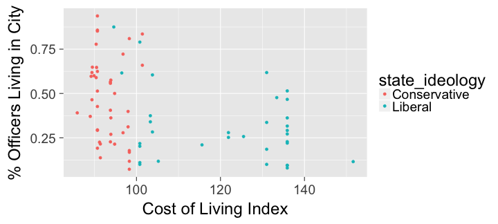<!-- --> --- ## Practice Use the 5MV to answer problems from R data packages, e.g., [`nycflights13` `\(\rightarrow\)` `weather`] <!-- Lay out what the resulting table should look like on paper first. --> 1. What is the maximum arrival delay for each carrier departing JFK? [`nycflights13` `\(\rightarrow\)` `flights`] 2. Calculate the domestic return on investment for 2013 scaled data descending by ROI <br> [`fivethirtyeight` `\(\rightarrow\)` `bechdel`] 3. Include the name of the `carrier` as a column in the `flights` data frame <br> [`nycflights13` `\(\rightarrow\)` `flights`, `airlines`] --- class: inverse, center, middle # DEMO in RStudio --- class: inverse, center, middle # Statistical Inference --- ## Statistical Inference We now enter the "traditional" topics of intro stats... 1. Sampling theory 1. Hypothesis testing 1. Confidence intervals 1. Regression --- ## Statistical Inference ... but now students are armed with 1. Data visualization 1. Data wrangling skills 1. **Most important**: comfort with coding! --- # Chapter 6: Sampling Highlights Sampling is at the root of statistics. Two approaches: <br> Either we use this... | Or we use this... :-------------------------:|:-------------------------: <img src="figure/formulas.png" alt="Drawing" style="width: 300px;"/> | <img src="figure/coding.jpg" alt="Drawing" style="width: 300px;"/> <br> --- ## `mosaic` Package It has functions for random simulations: <br> 1. `rflip()`: Flip a coin 1. `shuffle()`: Shuffle a set of values 1. `do()`: Do the same thing many, many, many times 1. `resample()`: the **swiss army knife** for sampling --- ## Lady Tasting Tea <center><img src="figure/lady_tasting_tea.jpg" alt="Drawing" style="height: 450px;"/></center> --- ## Presented to Students As: * Say you are a statistician and you meet someone called the "Lady Tasting Tea." * She claims she can tell by tasting whether the tea or the milk was added first to a cup. * You want to test whether + She can actually tell which came first + She's lying and is really guessing at random * Say you have just enough tea/milk to pour into 8 cups. --- ## Lady Tasting Tea The example will be built around this code: (Available in the supplementary HTML document [here](https://ismayc.github.io/moderndive-workshops/slides/slide_document.html#chapter_6:_sampling_highlights).) ```r library(ggplot2) library(dplyr) library(mosaic) single_cup_guess <- c(1, 0) simulation <- do(10000) * resample(single_cup_guess, size=8, replace=TRUE) View(simulation) simulation <- simulation %>% mutate(n_correct = V1 + V2 + V3 + V4 + V5 + V6 + V7 + V8) View(simulation) ggplot(simulation, aes(x=n_correct)) + geom_bar() + labs(x="Number of Guesses Correct", title="Number Correct Assuming She Is Guessing at Random") + geom_vline(xintercept=8, col="red") ``` --- # Chapter 7: Hypothesis Testing Highlights **There is only one test; it has 5 components**: 1. Define `\(H_0\)` and `\(H_A\)` 1. Define the test statistic `\(\delta\)` 1. Compute the observed test statistic `\(\delta^*\)` 1. Construct the null distribution either * Mathematically * **Via Simulation** 1. Compare `\(\delta^*\)` to null distribution to compute p-value --- ## There is Only One Test: Lady Tasting Tea 1. She is guessing at random vs she can tell which came first 1. Test statistic: Number out of 8 shes guesses right 1. Observed test statistic: 8 of 8. The red line! 1. Null distribution: (simulated) bar graph! 1. p-value: Very small! Above 0.36% --- ## There is Only One Test: Goodness-of-Fit 1. Observations fit expected distibution vs not 1. Test statistic: `\(\sum_{i=1}^{k}\frac{\left(\mbox{Obs}_i-\mbox{Exp}_i\right)^2}{\mbox{Exp}_i}\)` 1. Observed test statistic: Compute using data! 1. Null Distribution: (mathematically derived) <br> [Chi-Squared Dist'n](https://beta.rstudioconnect.com/connect/#/apps/2719/access). 1. Area to the right! --- ## There is Only One Test <center><img src="figure/ht.png" alt="Drawing" style="width: 700px;"/></center> - Created by [Allen Downey](http://allendowney.blogspot.com/2016/06/there-is-still-only-one-test.html) --- ## Two-Sample Permutation Test Posed to students: Did students with an even # of letters in last name do better than those with odd #? (Available in the supplementary HTML document [here](https://ismayc.github.io/moderndive-workshops/slides/slide_document.html#chapter_7:_hypothesis_testing_highlights).) ```r library(tidyverse) library(mosaic) grades <- read_csv("https://raw.githubusercontent.com/ismayc/moderndive-workshops/master/docs/slides/data/grades.csv") View(grades) # Observed Difference: Using mosaic package's mean function observed_diff <- mean(final ~ even_vs_odd, data=grades) %>% diff() null_distribution <- (do(1000) * mean(final ~ shuffle(even_vs_odd), data=grades)) %>% mutate(difference=odd-even) View(null_distribution) # Plot ggplot(data=null_distribution , aes(x=difference)) + geom_histogram(binwidth = 0.025) + labs(x="Avg of Odds - Avg of Evens") + geom_vline(xintercept = observed_diff, col="red") ``` --- # Chapter 8: Confidence Intervals Highlights * Not only show students repeated sampling (with a Shiny app for example), let them repeatedly sample! * In other words, let them construct sampling distributions. --- ## Sampling Distribution, SE, & C.I. Example The example will be built around this code: (Available in the supplementary HTML document [here](https://ismayc.github.io/moderndive-workshops/slides/slide_document.html#chapter_8:_confidence_intervals_highlights.)) 1. Discuss with your seatmates what all 5 code parts below are doing. 1. Try increasing `n` and repeating. What does this correspond to doing in real life? 1. How does the histogram change? 1. Describe using statistical language the role `n` plays when it comes to estimating `\(\mu\)`. <br><br> ```r library(ggplot2) library(dplyr) library(mosaic) library(okcupiddata) data(profiles) # For simplicity, remove 3 individuals who did not list their height profiles <- profiles %>% filter(!is.na(height)) # Population mean mu <- mean(profiles$height) # Sample size: n <- 5 # Parts 1 & 2: resample(profiles$height, size=n, replace=TRUE) mean(resample(profiles$height, size=n, replace=TRUE)) # Part 3: samples <- do(10000) * mean(resample(profiles$height, size=n, replace=TRUE)) View(samples) # Part 4: ggplot(samples, aes(x=mean)) + geom_histogram(binwidth = 1) + labs(x="sample mean") + xlim(c(50,80)) + geom_vline(xintercept=mu, col="red") # Part 5: sd(samples$mean) ``` --- ## The Hard Part Convincing students: * We only do the blue via simulation *as a theoretical exercise* * We do the purple in *real life* <br> <center><img src="figure/SE.png" alt="Drawing" style="width: 800px;"/></center> --- # Chapter 9: Regression Highlights 1. Experience with `ggplot2` package and knowledge of the Grammar of Graphics primes students for regression 1. Use of the `broom` package to unpack regression --- ## 1. `ggplot2` Primes Regression * Mapping aesthetics to variables provides a natural framework for all of data visualization. Understanding the relationships between variables is clear and transparent from the `ggplot2` code. * This ultimately what regression is about! --- ## 1. `ggplot2` Primes Regression Example: * All Alaskan Airlines and Frontier flights leaving NYC in 2013 * We want to study the relationship between temperature and departure delay * For summer (June, July, August) and non-summer months separately Involves four variables: - `carrier`, `temp`, `dep_delay`, `summer` --- ## 1. `ggplot2` Primes Regression <!-- --> --- ## 1. `ggplot2` Primes Regression Why? Dig deeper into data. Look at `origin` and `dest` variables as well: <br> ``` Source: local data frame [2 x 4] Groups: carrier, origin [?] carrier origin dest `Number of Flights` <chr> <chr> <chr> <int> 1 AS EWR SEA 712 2 F9 LGA DEN 675 ``` --- ## 2. `broom` Package * The `broom` package takes the messy output of built-in modeling functions in R, such as `lm`, `nls`, or `t.test`, and turns them into tidy data frames. * Fits in with `tidyverse` ecosystem * This works for [many R data types](https://github.com/tidyverse/broom#available-tidiers)! --- ## 2. `broom` Package In our case, `broom` functions take `lm` objects as inputs and return the following in tidy format! * `tidy()`: regression output table * `augment()`: point-by-point values (fitted values, residuals, predicted values) * `glance()`: scalar summaries like `\(R^2\)`, --- ## 2. `broom` Package The chapter will be built around this code: (Available in the supplementary HTML document [here](https://ismayc.github.io/moderndive-workshops/slides/slide_document.html#chapter_9:_regression_highlights)). ```r library(ggplot2) library(dplyr) library(nycflights13) library(knitr) library(broom) set.seed(2017) # Load Alaska data, deleting rows that have missing departure delay # or arrival delay data alaska_flights <- flights %>% filter(carrier == "AS") %>% filter(!is.na(dep_delay) & !is.na(arr_delay)) %>% sample_n(50) View(alaska_flights) # Exploratory Data Analysis---------------------------------------------------- # Plot of sample of points: ggplot(data = alaska_flights, mapping = aes(x = dep_delay, y = arr_delay)) + geom_point() # Correlation coefficient: alaska_flights %>% summarize(correl = cor(dep_delay, arr_delay)) # Add regression line ggplot(data = alaska_flights, mapping = aes(x = dep_delay, y = arr_delay)) + geom_point() + geom_smooth(method = "lm", se = FALSE, color = "red") # Fit Regression and Study Output with broom Package--------------------------- # Fit regression delay_fit <- lm(formula = arr_delay ~ dep_delay, data = alaska_flights) # 1. broom::tidy() regression table with confidence intervals and no p-value stars regression_table <- delay_fit %>% tidy(conf.int=TRUE) regression_table %>% kable(digits=3) # 2. broom::augment() for point-by-point values regression_points <- delay_fit %>% augment() %>% select(arr_delay, dep_delay, .fitted, .resid) regression_points %>% head() %>% kable(digits=3) # and for prediction new_flights <- data_frame(dep_delay = c(25, 30, 15)) delay_fit %>% augment(newdata = new_flights) %>% kable() # 3. broom::glance() scalar summaries of regression regression_summaries <- delay_fit %>% glance() regression_summaries %>% kable(digits=3) # Residual Analysis------------------------------------------------------------ ggplot(data = regression_points, mapping = aes(x = .resid)) + geom_histogram(binwidth=10) + geom_vline(xintercept = 0, color = "blue") ggplot(data = regression_points, mapping = aes(x = .fitted, y = .resid)) + geom_point() + geom_abline(intercept = 0, slope = 0, color = "blue") ggplot(data = regression_points, mapping = aes(sample = .resid)) + stat_qq() # Preview of Multiple Regression----------------------------------------------- flights_subset <- flights %>% filter(carrier == "AS" | carrier == "F9") %>% left_join(weather, by = c("year", "month", "day", "hour", "origin")) %>% filter(dep_delay < 250) %>% mutate(summer = ifelse(month == 6 | month == 7 | month == 8, "Summer Flights", "Non-Summer Flights")) ggplot(data = flights_subset, mapping = aes(x = temp, y = dep_delay, col = carrier)) + geom_point() + geom_smooth(method = "lm", se = FALSE) + facet_wrap(~summer) ``` --- class: inverse, center, middle # The Future of ModernDive <u>Recall</u>: Slides at <http://bit.ly/uscots17-slides> <br> Supplementary HTML document at <br> <http://bit.ly/uscots17-html> --- ## The Immediate Future By July 1st, 2017 * Complete Development of Chapters 6-9 on Simulations, Hypothesis Testing, Confidence Intervals, and Regression * Learning Checks: Discussion/solutions embedded directly in the textbook, that you can reveal progressively. * Have better [data frame printing](http://rmarkdown.rstudio.com/html_document_format.html#data_frame_printing). Instead of raw R code use + Less jarring `knitr::kable()` output or + Interactive table outputs, to partically replicate RStudio's `View()` function. --- ## The Longer Term * In Chapter 9: Regression + Add more on categorical predictors + Multiple regression --- ## The Longer Term ## DataCamp - Continue to build supplementary materials for other disciplines - [Effective Data Storytelling using the tidyverse](https://www.datacamp.com/courses/effective-data-storytelling-using-the-tidyverse) designed for Social Scientists/Data Journalists - Add [DataCamp Light](https://github.com/datacamp/datacamp-light) chunks into the book to enable student practice right there inside the textbook via the `tutorial` [package](https://github.com/datacamp/tutorial) --- ## The Longer Term ## Implement Cognitive Science Research - Work on interleaving and spaced practice inside the textbook to improve student learning and retention - Follow the [principles and research](http://www.learningscientists.org/posters) laid out by the [Learning Scientists](http://www.learningscientists.org/) --- ## The Longer Term ## Further Develop Interactive Applets - To help students visualize and understand inferential processes - [Sampling app](https://ismay.shinyapps.io/okcupidheights/) - [Probability Distribution Viewer and Calculator](http://ismay.shinyapps.io/ProbApp) - (MAYBE) Learn D3.js and create applets like those at <br> [Seeing Theory](http://students.brown.edu/seeing-theory/) --- class: inverse, center, middle ## Introduction to `bookdown` --- ## What is Markdown? - A "plaintext formatting syntax" - Type in plain text, render to more complex formats - One step beyond writing a `txt` file - Render to HTML, PDF, DOCX, etc. using Pandoc --- ## What does it look like? .left-column[ ``` # Header 1 ## Header 2 Normal paragraphs of text go here. **I'm bold** [links!](http://rstudio.com) * Unordered * Lists And Tables ---- ------- Like This ``` ] .right-column[ <img src="figure/markdown.png" alt="markdown" style="width: 270px;"/> ] --- ## What is R Markdown? - "Literate programming" - Embed R code in a Markdown document - Renders textual output along with graphics *** .left-column[ ``` ` ` `{r chunk1} library(ggplot2) library(nycflights13) pdx_flights <- flights %>% filter(dest == "PDX", month == 5) nrow(pdx_flights) ` ` ` ` ` `{r chunk2} ggplot(data = pdx_flights, mapping = aes(x = arr_delay, y = dep_delay)) + geom_point() ` ` ` ``` ] .right-column[ ``` [1] 88 ``` <!-- --> ] --- ## What is `bookdown`? From [bookdown book about `bookdown`](https://bookdown.org/yihui/bookdown/): > Author books with R Markdown, including generating figures and tables, and inserting cross-references, citations, HTML widgets, and Shiny apps in R Markdown. The book can be exported to HTML, PDF, and e-books (e.g. EPUB). The book style is customizable. You can easily write and preview the book in RStudio IDE or other editors, and host the book wherever you want (e.g. bookdown.org). --- ## The Basics of `bookdown` - `index.Rmd` file is the "driver" - `Rmd` files numbered in the order you want them to appear in the book - `_bookdown.yml` gives output specifications - **Set `output_dir: "docs"` to work with GitHub Pages** - `_output.yml` provides which types of output (webpage, PDF, Word Document, epub) to produce (with arguments) - We will focus on webpage/gitbook --- class: inverse, center, middle # DEMO of `bookdown` <br> with ModernDive Light --- ## Uploading to GitHub Pages * Create a [GitHub Pages](https://pages.github.com/) personal page. Ex: [rudeboybert.github.io](rudeboybert.github.io) * Create New Repository * Follow instructions in 2nd paragraph of [Authoring Books and Technical Documents with R Markdown](https://bookdown.org/yihui/bookdown/github.html) * Drag and drop onto GitHub repository using "Upload Files" Button --- class: middle # Thanks for attending! - [Workshop Feedback Form](https://goo.gl/forms/EOEYWAd8jg04QVf72) - Email us if you'd like to chat further during USCOTS or later - [chester@moderndive.com](mailto:chester@moderndive.com) / [albert@moderndive.com](mailto:albert@moderndive.com) - [Source code for ModernDive](https://github.com/ismayc/moderndiver-book) - Feel free to modify the book as you wish for your own needs! Just please list the authors as "Chester Ismay, Albert Y. Kim, and YOU!" - These slides available [here](http://bit.ly/uscots2017-slides) - Slides created via the R package [xaringan](https://github.com/yihui/xaringan) by Yihui Xie - Source code for these slides at <https://github.com/ismayc/moderndive-workshops>